Dynamic Evaluation of Enterprise Risk Management at Eletrobras Furnas in Brazil¹

• By Admin
• March 4, 2015
• Comments Off on Dynamic Evaluation of Enterprise Risk Management at Eletrobras Furnas in Brazil¹

This white paper is intended to describe the methodology applied in automating Enterprise Risk Management (ERM) for Eletrobras Furnas, the largest utility company in Brazil. The ERM approach uses Real Options Valuation, Inc. (ROV) PEAT software’s ERM module, and adapts the Risk Matrix model currently used by the Eletrobras group to the concept of expected value of risk, pushing the envelope from qualitative risk assessment to more quantitative risk management.

Introduction

The PEAT ERM module was built according to the concept of Expected Risk, which uses the concept of quantification of risks, enabling plans for risk mitigation, statistical evaluation, strategic real options, and analysis of alternatives, as well as optimizing the portfolios of multiple projects. PEAT has over 20 U.S. and international patents and patents pending protection on its sophisticated analytics and approach to Integrated Risk Management methodologies. See the PEAT ERM Whitepaper for more technical details on the software applications and functionalities.

To get started, ERM requires a two‐dimensional input of Likelihood (L) or Frequency of a risk event occurring and Impact (I) or the Severity in terms of financial, economic, and noneconomic effects of the risk.  These L and I concepts are industry standard and used even in regulatory environments such as the Basel II and Basel III Accords (initiated by the Bank of International Settlements in Switzerland and accepted by most Central Banks around the world as regulatory reporting standards for operational risks).

However , Eletrobras is a utility company and is not subject to stringent banking and  financial regulations;  therefore, in place of the probability scale of Likelihood or Frequency, Eletrobras uses the concept of Vulnerability (V). Consequently, the typical ERM risk matrix is modified slightly as shown in Figure1.

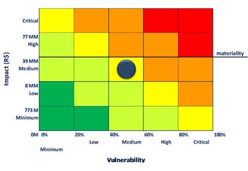
Using Likelihood or Vulnerability is similar and the choice of which to use is entirely up to the organization. However, we do observe several advantages of using the concept of Vulnerability, especially as it facilitates the existing audit activity in Eletrobras because the degree of vulnerability metric within the company has already been associated with the evaluation of easily auditable controls and has been in use for several years.

This whitepaper explores how the PEAT ERM module was customized and applied at Eletrobras, allowing its managers to not only document the major risk factors but to also push the envelope of risk analytics and perform sensitivity analysis, Monte Carlo risk simulation, and quantitative analytics and to assess the dynamics of its business risks, risk controls, and overall enterprise risk management. For the sole purpose of this whitepaper, we will adapt and use the concept of Vulnerability associated with items related to internal control standards and guidelines already established in Brazil and internationally (e.g., ISO‐31000, COSO, COBIT, and SOX or Sarbanes‐Oxley Act). The purpose of this customization is to make it possible to qualify and quantify the degree of implementation in each of the Risk Elements (RE) attached to specific Eletrobras’ companywide programs.

Uncertainty, Risk, and Vulnerability

In enterprise risk assessment of the quantitative risk environment, the concept of uncertainty is associated with the Likelihood (L) of an event happening in the future. The uncertainties of repetitive events observed in nature over a long period of time can sometimes become predictable but usually not with absolute certainty. Such observances can be associated with mathematical functions that reflect the statistical properties of something likely to occur at a future time.

The risk of an event occurring is connected to two parameters: the Impact (I) caused by an uncertain event and the probability of an event occurring or its Likelihood (L). Given some known probability of a risk event occurring, the higher the impact, the greater the risk. If the impact is zero, the risk will be zero even though the event has a high probability of occurring. The reverse argument is also true. If the probability of a risk event occurring is equal to zero, the risk is zero (this is an environment of pure certainty), regardless of the magnitude of the impact.

In other words, uncertainty is measured in terms of Likelihood of occurrence, and unless there is some financial or noneconomic but observable Impact, there is no risk, just uncertainty.

Within the realm of Eletrobras, the concept of Vulnerability (V) is associated with the risk of an event. Put another way, Vulnerability is associated with an organization’s susceptibility to the consequences of a risk event. Risk is reduced through the mitigation of risk, either by decreasing the Likelihood of an event occurring (e.g., rather than leaving the car parked on a deserted street at night, put it in a garage under camera surveillance) or by reducing its Impact (e.g., purchasing auto theft insurance) to protect your capital.

The mitigation of the risk consequences can be scaled according to the predictable value of risk. For example, say we have a specific risk event where its maximum financial impact is valued at $100, with a 10% probability of occurring. Further suppose that there is a minimum or residual value of $5 with 90% probability, which implies that there is an expected value of $14.5. Thus, mitigation measures can be designed to try to neutralize this exposure. Clearly, there are two ways to reduce the risk: reduce the Impact or reduce the Likelihood.

Impact reduction means taking preventive measures (e.g., entering into contractual agreements to reduce legal liability), and Likelihood reduction may mean changing organizational processes and behaviors (e.g., changing processes that have a high probability of disaster). Nevertheless, regardless of the steps used to reduce the Likelihood or Impact, if the possibility still exists of the risk event occurring, the risk should be assessed on two levels: the mitigated risk and the residual risk. Mitigation measures are meant to reduce the first level of risk to its residual risk whenever possible.

Proposed Mechanism for Dynamic Risk Indicators

Institutional rules or guidelines that address business risk with only a qualitative view do not indicate a method to evaluate this exposure quantitatively. In the traditional qualitative analysis, the measure of the riskiness of a company is a snapshot at a point in time. Mitigation measures are evaluated later, often from audits to verify the degree of compliance on previous snapshots. The effort to implement these mitigation measures is typically not dynamically evaluated, nor are its results compared to what was expected within the range of risks vis‐à‐vis the cost of mitigation.

The PEAT ERM module intends not only to document the state of vulnerability of a company to the events that may lead to risk losses, whether economic or noneconomic, but also to quantify and measure the uncertainties of the risks and their mitigation costs.  All of this is done dynamically, whereby the company may periodically make adjustments to achieve its targeted goals for reducing exposure, and pushes the envelope from qualitative assessment to quantitative risk analysis.

PEAT ERM allows dynamic assessments and measures the degree of vulnerability of the company over time using the “% Mitigation Completed” parameter for each risk control and their respective weights in the Risk Register window (see Figure 5), which assumes the function of the measurement parameter of Vulnerability as applied within Eletrobras. This percentage parameter is interpreted as “% Mitigation Completed = 100% − % Vulnerability” indicating a reduction in risk exposure due to the company having implemented measures to reduce its exposure to the risks identified.

This parameter ranges from 0% Complete (i.e., 100% Vulnerable), indicating that the company is exposed to the Total Risk Value, up to 100%; whereas a 100% Complete indicates a 0% Vulnerability measure, where the risk is reduced to an exposure at its minimum level, also known as the Residual Value Risk.

Accounting for Corporate Risk

The set of Key Risk Indicators (KRI) provides an overview of financial risk to which the company is subject. Figure 2 shows an example of the residual risk exposure in PEAT ERM. In the following example, we present the risk exposure of the Finance Department due to the Risk Element of Cost Overrun. In the example, the Gross Value of Risk is $1,000,000 and its Residual Value is $500,000. The Corporate Risk, composed of all the risk factors of the company, is $1,480,000.

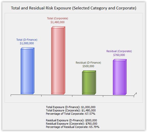
In this example, KRI Overrun is measured as (L = 4) * (I or V = 4) = (KRI = 16) and can be shown in the Risk Matrix. In this case, it is classified as a Moderate Risk, and a reduction factor of 50% will reduce the risk exposure to $750,000 or a KRI of 12.

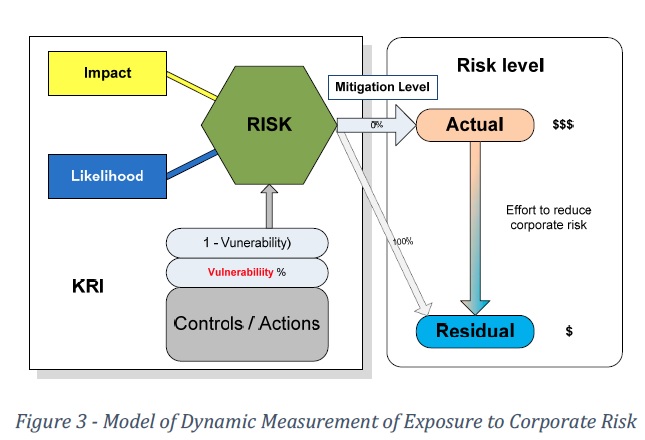
The model of dynamic measurement of exposure to corporate risk has the graphical representation as shown in Figure 3.

In this case, the company can assess its risk exposure dynamically by implementing the mitigation of Risk Factors, which may be marked by international standards and controls (e.g., SOX, COBIT). Thus, the Vulnerability used by Eletrobras is associated with compliance with the controls. Dynamically this can be represented by Figure 4.

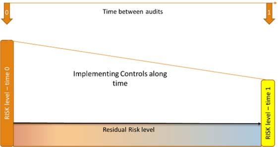
By means of the audit, be it external or internal, the company can show the evolution of the measures taken to mitigate the risk and reduce the financial exposure of the company.

Dynamic Assessment of Vulnerability: An Illustration

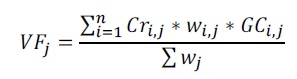
The Vulnerability Factor (VF) is associated with a set of controls (Cri,j), based on international standards or internal rules that must be fulfilled to reduce the Risk Element REj to a level of residual risk. Each control (Cri,j) by REj selected should be associated with a weight (wi,j) equal to one, two, or four, depending on the degree of importance attached to it. The use of weights allows us to distinguish between controls that are more difficult to be implemented or which would have a much greater impact on risk mitigation. Our suggestion is to rank the controls by the degree of impact: minor impact should be classified as having a weight identical to unity; the average impact of a weight equal to 2 (two); and, finally, if any, high impact with weight 4 (four), providing a sense of geometric growth.

After an audit, controls may have different degrees of conformity (GCi,j), namely implemented (0%), partially implemented (50%), and nondeployed (100%). The REj audited Vulnerability Factor (VFi,j) is calculated using the following formula:

Case Illustration

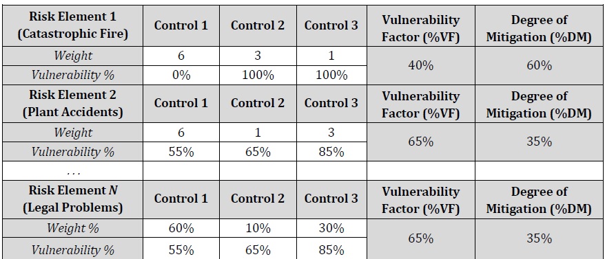
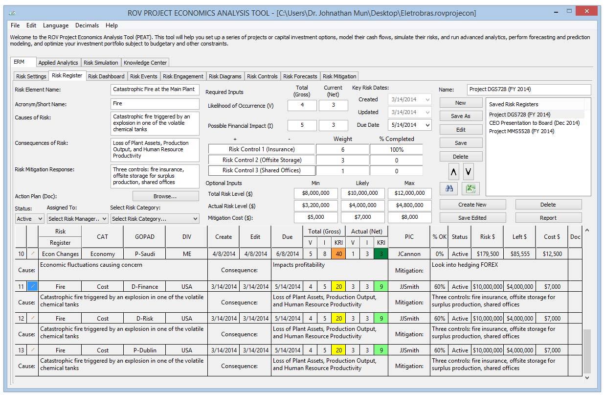
Figure 5 illustrates a manual computation of several sample Risk Elements, their respective Risk Controls, Weights, Vulnerability %, and the computed Vulnerability Factor (%VF) and Degree of Mitigation (%DM). It also shows a screen shot of the PEAT ERM Risk Register tab showing how these assumptions can be entered and the subsequent simple steps to set up the ERM Risk Register.

Explanation Details

• A Risk Register comprises multiple Risk Elements. Figure 5’s PEAT ERM shows three sample saved Risk Registers, with the highlighted Risk Register being actively edited (e.g., Project DGS728).
• A Risk Element means an actual or anticipated risk. In the table, we see there are n Risk Elements in a single Risk Register. The first Risk Element example is a catastrophic fire risk event at one of the plants or utility facilities, another risk is employee accidents at the plants (Risk Element 2), and so forth, ending with legal risks (Risk Element N).
• In the first Risk Element, the catastrophic fire, let’s say, for illustration purposes, there are
  three problems relating to this fire: destruction and loss of assets (Assets), loss of production and output (Production), and loss of human productivity (Productivity).
• Each problem is mitigated by a control. Control 1 mitigates losses in Assets by purchasing fire insurance; Control 2 mitigates losses in Production by installing capacitors and storage areas in a different off‐site location that can store excess production and handle demand for the next 90 days after a catastrophic fire; and Control 3 mitigates Productivity losses by initiating a joint venture with a partner company to house all the employees at a temporary workplace while at the same time migrating all IT systems to a cloud‐based environment for instant restoration of proprietary data such that employees can get back to work almost immediately.
• Let’s further assume a simple scenario involving Risk Element 1 where the estimated total and complete catastrophic fire event will mean a loss of $6M in Assets, $3M in Production, and $1M in Productivity. These amounts were obtained through an audit by the risk
  personnel by performing inventory of the assets, financial analysis of production rates and loss revenues, and human resource estimations. Using these estimates, we can enter the relevant weights, either as numerical values or percentages. For instance, Control 1 has a weight of 6, Control 2 has a weight of 3, and Control 3 has a weight of 1, commensurate with the total gross risk covered and mitigated by each control for this single Risk Element. Of course, each company may have its own paradigm in setting the weights, as long as it is consistent throughout its ERM implementation. In this simple example we look at weighting the risk‐reduction impact, whereas different organizations who do not have such impact numbers may similarly use degree of difficulty to execute the control, complication, or cost to implement (in which case the weights will be different than in the example above).
• Furthering our example, let’s say that Control 1 (fire insurance) is very simple to execute and coverage was already purchased for the full amount of the Assets, which means that the % Mitigation Completed (%M) is 100% or, alternatively, % Vulnerability (%V) is 0%. Controls 2 and 3 are more difficult to complete and take time and money, and, as of right now, they are 0% completed (0% mitigated or 100% vulnerable if a fire occurs).
• As a side note, %M and %V are complementary to each other (i.e., 1 – %V = %D), and expressing either vulnerability or degree of mitigation is a matter of preference (%M takes a more optimistic point of view whereas %V takes a more pessimistic point of view, but converting from one measure to another is very simple as described).
• See the table for Risk Element 2 (employee accidents at the plant) for another sample set of inputs. Finally, Risk Element N intentionally showcases the same weighting levels but here a percentage weight is used instead. Therefore, instead of a numerical weight of 6, 1, 3 (which sums to 10), we can alternatively input these as 60%, 10%, and 30% (this is equivalent to 6/10, 1/10, and 3/10). This is a user preference and can be set in PEAT ERM’s Global Settings tab.
• Then, the PEAT ERM module automatically computes the Vulnerability Factor (%VF) and Degree of Mitigation (%DM) for each of the Risk Elements. The following shows their respective calculations:
  • Risk Element 1: Catastrophic Fire.
    • %VF=(6X0%+3X100%+1X100%)/(6+3+1)=40%
    • %DM=1-%VF=100%-40%=60%, or similarly we have
    • %DM=1-(6X0%+3X100%+1×100%)/(6+3+1)=60%
  • Risk Element 2: Plant Accidents.
    • %VF=(6X55%+1×65%+3×85%)/(6+1+3)=65%
    • %DM=1-%VF=100%-65%=35%, or , similarly, we have :
    • %DM=1-(6X55%+1×65%+3×85%)/(6+1+3)=35%
• Risk Element N: Legal Issues. In this example, we use % weights instead.
  • %VF=(60%x55%+10%x65%+30%x85%)=65%
  • %DM=1-%VF=100%-65%=35%,or, similarly, we have:
  • %DM=1-(60%x55%+10%x65%+30%x85%)=35%
• As a side note, the numerical weight can take on any positive integer and does not have any further restrictions, whereas the % weight each needs to be between 0% and 100%, and the total weights for each Risk Element must sum to 100%.
• The monetary Gross Risk for Risk Element 1 (catastrophic fire) is, of course, $6M + $3M + $1M = $10M. And in the example above, we see that only Control 1 (fire insurance) was 100% mitigated (0% vulnerable). This means the entire $6M has been mitigated and the
  risk no longer exists, at least financially speaking. Thus, the Remaining or Residual Risk is $3M + $1M = $4M. Alternatively, we can compute the Residual Risk=Gross Risk x %vulnerability factor Of course, this is the same as saying Residual Risk= Gross Risk x (1-% Degree of Mitigation). That is, we can compute Residual Risk = $10M x 40%=$10Mx(1-60%)=$4M This $4M is the Remaining or Residual Risk or the risk that remains after the Risk Controls are in place. As a side note, COSO requirements specifically state to use Impact and Likelihood measures and define Gross Risk as Inherent Risk, and Residual Risk as the remaining risks after management executes whatever controls they have executed. (See Dr. Johnathan Mun’s Modeling Risk, Third Edition’s Chapter 16 for specifications of how PEAT complies with Basel II/III, ISO 31000:2009, and COSO global standards.) Regardless of the definitions used in the example here, clearly, different companies have different paradigms; the important things is to be consistent in defining them. If we compute the Remaining Risk in the example above, the user has the option to change the name “Residual Risk” to something like “Actual or Remaining Risk” in the PEAT ERM’s Global Settings tab to avoid any confusion.

Procedures

The following shows how simple it is to use PEAT ERM to input Risk Elements and Risk Controls into a Risk Register (Figure 5):

• Step 1: In the relevant Risk Register, users can input new Risk Elements in the data grid or edit an existing Risk Element (click on the pencil icon in the data grid for the relevant row to edit). Each Risk Element is shown as a new row in the Risk Register’s data grid.
• Step 2: Enter the Risk Controls, Weight, and % Mitigation Completed for each control item (weights can be entered as integers or percent depending on user settings in the Global Settings tab). The % Degree of Mitigation is automatically computed and shown in the data grid under the %OK column.
• Step 3: Users can optionally enter the monetary Gross Risk amounts if required and known, as well as a spread that will be used later in running Monte Carlo risk simulations. For instance, enter $8M, $10M, and $12M, where the most likely Gross Risk is $10M as illustrated in this example (the sum of the Assets, Production, and Productivity).
• Step 4: Users can then optionally enter the monetary Residual Risk amounts if required. This is very simple to enter: simply take the Gross Risk amounts and multiply by (1 – %DM). In this example, the Residual Risk spreads will be:
  • Minimum Residual Risk=$8 M x(1-60%)=$3.2 M
  • Most likely Residual Risk=$10 M x(1-60%)=$4.0 M.
  • Maximum Residual Risk =$12 M x (1-60%)=$4.8 M
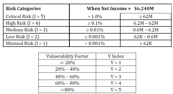
• Step 5: Depending whether the user has previously selected the Impact and Vulnerability or the Impact and Likelihood settings for the Risk Matrix in the Global Settings tab of PEAT ERM, users can either use the $4M computed Actual Risk or Residual Risk amount or the %OK (i.e., % Vulnerability Factor for the Risk Element after performing the weighted average computation of the various Risk Controls), or they can use their own specified categories and enter either the V or I value. For example, the following is an example of companyspecific V and I values, which can be tied to net income, revenues, or other metrics, and are obviously unique to each company and may change over time. These categorizations will be decided by the company’s risk committee (the example below is for a 5 × 5 risk matrix):

Step 6: Continue adding more Risk Elements in the Risk Register, perform tornado, scenario, and simulation analysis, as well as run the various Risk Dashboard reports.

Dynamic Evaluation of Impact, Probability, and KRI

The impact is always associated with the wealth of the decision maker. For example, a company that moves billions of dollars every month in its business of mining or oil extraction has a very different risk appetite than a bakery or pharmacy. The levels of impact designed in the Risk Matrix should be associated with the appropriate financial impact scale. These financial ranges can be indexed, for example, to the turnover of the company, so that the monetary values of risk are related to or are always updated with the size of the company, since the KRIs are absolute and its evolution will depend only on the implementation of the risk mitigation measures and the nonvolatile wealth of the company. In contrast, the probability of an event is associated with a measure of whether it will occur regardless of the actions of the company’s managers. It may be the result of a Monte Carlo risk simulation (in the case of measuring the VaR [Value at Risk] or other associated probability and confidence intervals) or a subjective evaluation of those responsible for its management. Usually, experts have some sensitivity, based on their experience, about the chances of a risk event occurring. This value can then be the result of an analytical assessment or research and expert consensus.

A quantitative assessment of the risk or the KRI is associated with mitigation or reduction of risk exposure. These measures can be understood or organized in a listed group, whereby risks are assessed as “OK” or “Low” so that these events, if they occur, are not relevant to the financial health or the image of the company, or are very severe and may compromise the survival of the company. The group’s risk managers should define measures of exclusion or mitigation of risks so that they are always on the “Critical” to “Acceptable” level, and the level of investment to be made by the company in mitigating actions should be less than the decrease of the expected risk.

_______________________________________________________________________________________________
¹This whitepaper was written by Dr. Nelson Albuquerque and Dr. Johnathan Mun. The authors acknowledgeand appreciate the collaboration of Eletrobras Furnas SA, which allowed us access to this enterprise riskmanagement project and its officers, Welington Cristiano Lima and José Roberto Teixeira Nunes, and for the thorough review conducted by Professor Pedro Bello, also of Eletrobras.