EXTREME VALUE THEORY AND APPLICATION TO MARKET SHOCKS FOR STRESS TESTING AND EXTREME VALUE AT RISK

• By Admin
• March 25, 2015
• Comments Off on EXTREME VALUE THEORY AND APPLICATION TO MARKET SHOCKS FOR STRESS TESTING AND EXTREME VALUE AT RISK

Economic Capital is highly critical to banks (as well as central bankers and financial regulators who monitor banks) as it links a bank’s earnings and returns on investment tied to risks that are specific to an investment portfolio, business line, or business opportunity. In addition, these measurements of Economic Capital can be aggregated into a portfolio of holdings. To model and measure Economic Capital, the concept of Value at Risk (VaR) is typically used in trying to understand how the entire financial organization is affected by the various risks of each holding as aggregated into a portfolio, after accounting for pairwise cross-correlations among various holdings. VaR measures the maximum possible loss given some predefined probability level (e.g.,99.90%) over some holding period or time horizon (e.g., 10 days). Senior management and decision makers at the bank usually select the probability or confidence interval, which reflects the board’s risk appetite, or it can be based on Basel III capital requirements. Stated another way, we can define the probability level as the bank’s desired probability of surviving per year. In addition, the holding period usually is chosen such that it coincides with the time period it takes to liquidate a loss position.

VaR can be computed several ways. Two main families of approaches exist: structural closed-form models and Monte Carlo risk simulation approaches. We showcase both methods later in this case study, starting with the structural models. The second and much more powerful of the two approaches is the use of Monte Carlo risk simulation. Instead of simply correlating individual business lines or assets in the structural models, entire probability distributions can be correlated using more advanced mathematical Copulas and simulation algorithms in Monte Carlo risk simulation methods by using the Risk Simulator software. In addition, tens to hundreds of thousands of scenarios can be generated using simulation, providing a very powerful stress testing mechanism for valuing VaR. Distributional fitting methods are applied to reduce the thousands of historical data into their appropriate probability distributions, allowing their modeling to be handled with greater ease.

There is, however, one glaring problem. Standard VaR models assume an underlying Normal Distribution. Under the normality assumption, the probability of extreme and large market movements is largely underestimated and, more specifically, the probability of any deviation beyond 4 sigma is basically zero. Unfortunately, in the real world, 4-sigma events do occur, and they certainly occur more than once every 125 years, which is the supposed frequency of a 4-sigma event (at a 99.995% confidence level) under the Normal Distribution. Even worse, the 20-sigma event corresponding to the 1987 stock crash is supposed to happen not even once in trillions of years.

The VaR failures led the Basel Committee to encourage banks to focus on rigorous stress testing that will capture extreme tail events and integrate an appropriate risk dimension in banks’ risk management. For example, the Basel III framework affords a bigger role for stress testing governing capital buffers. In fact, a 20-sigma event, under the Normal Distribution, would occur once every googol, which is 1 with 100 zeroes after it, years. In 1996, the Basel Committee had already imposed a multiplier of four to deal with model error. The essential non-Normality of real financial market events suggests that such a multiplier is not enough. Following this conclusion, regulators have said VaR-based models contributed to complacency, citing the inability of advanced risk management techniques to capture tail events.

Hervé Hannoun, Deputy General Manager of the Bank for International Settlements, reported that during the crisis, VaR models “severely” underestimated the tail events and the high loss correlations under systemic stress. The VaR model has been the pillar for assessing risk in normal markets but it has not fared well in extreme stress situations.Systemic events occur far more frequently and the losses incurred during such events have been far heavier than VaR estimates have implied. At the 99% confidence level, for example, you would multiply sigma by a factor of 2.33.1

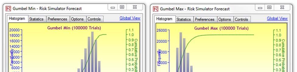
While a Normal Distribution is usable for a multitude of applications, including its use in computing the standard VaR where the Normal Distribution might be a good model near its mean or central location, it might not be a good fit to real data in the tails (extreme highs and extreme lows), and a more complex model and distribution might be needed to describe the full range of the data. If the extreme tail values (from either end of the tails) that exceed a certain threshold are collected, you can fit these extremes to a separate probability distribution. There are several probability distributions capable of modeling these extreme cases, including the Gumbel Distribution (also known as the Extreme Value Distribution Type I), the Generalized Pareto Distribution, and Weibull Distribution. These models usually provide a good fit to extremes of complicated data.

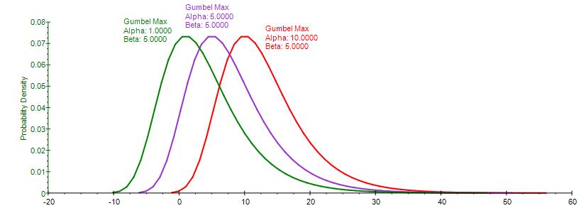
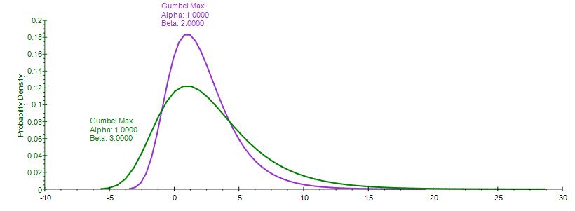
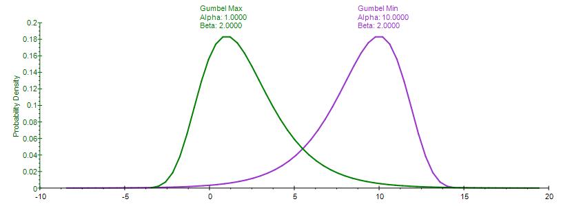
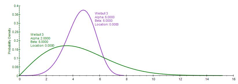
Figure 1 illustrates the shape of these distributions. Notice that the Gumbel Max (Extreme Value Distribution Type I, right skew), Weibull 3, and Generalized Pareto all have a similar shape, with a right or positive skew (higher probability of a lower value, and a lower probability of a higher value). Typically, we would have potential losses listed as positive values (a potential loss of ten million dollars, for instance, would be listed as $10,000,000 losses instead of – $10,000,000 in returns) as these distributions are unidirectional. The Gumbel Min (Extreme Value Distribution Type I,left skew), however, would require negative values for losses (e.g., a potential loss of ten million dollars would be listed as –$10,000,000 instead of $10,000,000). See Figure 4 for an example dataset of extreme losses. This small but highly critical way of entering the data to be analyzed will determine which distributions you can and should use.

 

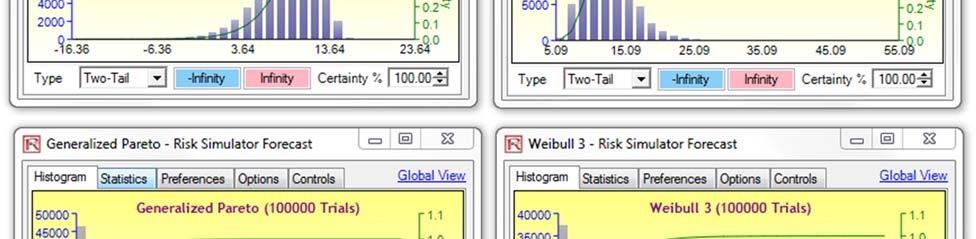
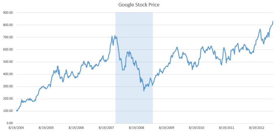
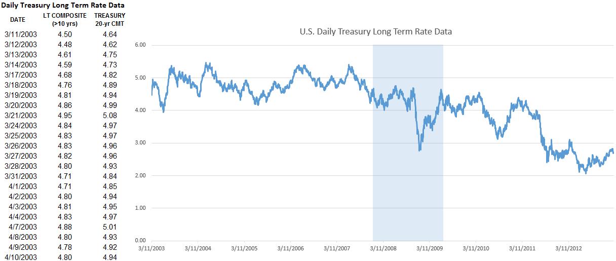
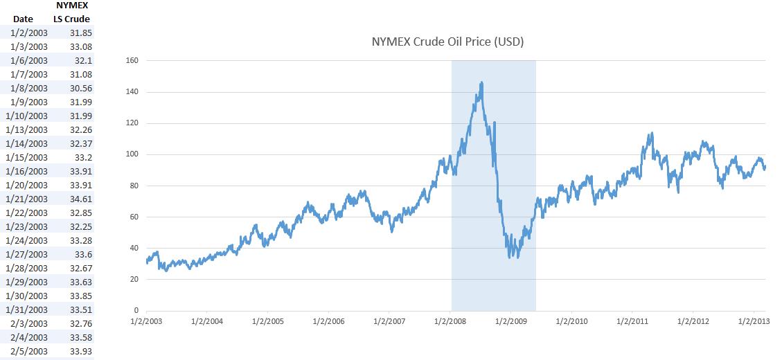
The probability distributions and techniques shown in this case study can be used on a variety of datasets. For instance, you can use extreme value analysis on stock prices (Figure 2) or any other macroeconomic data such as interest rates or price of oil, and so forth (Figure 3 illustrates historical data on U.S. Treasury rates and global Crude Oil Prices for the past 10 years). Typically, macroeconomic shocks (extreme shocks) can be modeled using a combination of such variables. For illustration purposes, we have selected Google’s historical stock price to model. The same approach can be applied to any time-series macroeconomic data. Macroeconomic shocks can sometimes be seen on time-series charts. For instance, in Figures 2 and 3, we see the latest U.S. recession at or around January 2008 to June 2009 on all three charts (highlighted vertical region).

 

Therefore, the first step in extreme value analysis is to download the relevant time-series data on the selected macroeconomic variable. The second step is to determine the threshold––data above and beyond this threshold is deemed as extreme values (tail ends of the distribution)—where these data will be analyzed separately.

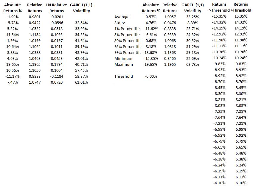
Figure 4 shows the basic statistics and confidence intervals of Google stock’s historical returns. As an initial test,we select the 5th percentile (–6.61%) as the threshold. That is, all stock returns at or below this –6.00% (rounded) threshold are considered potentially extreme and significant. Other approaches can also be used such as (i) running a GARCH model, where this Generalized Autoregressive Conditional Heteroskedasticity model (and its many variations) is used to model and forecast volatility of the stock returns, thereby smoothing and filtering the data to account for any autocorrelation effects; (ii) creating Q-Q quantile plots of various distributions (e.g., Gumbel, Generalized Poisson, or Weibull) and visually identifying at what point the plot asymptotically converges to the horizontal; and (iii) testing various thresholds to see at what point these extreme value distributions provide the best fit. Because the last two methods are related, we only illustrate the first and third approaches

Figure 4 shows the filtered data where losses exceed the desired test threshold. Losses are listed as both negative values as well as positive (absolute) values. Figure 5 shows the distributional fitting results using Risk Simulator’s distributional fitting routines applying the Kolmogorov-Smirnov test.

 

 

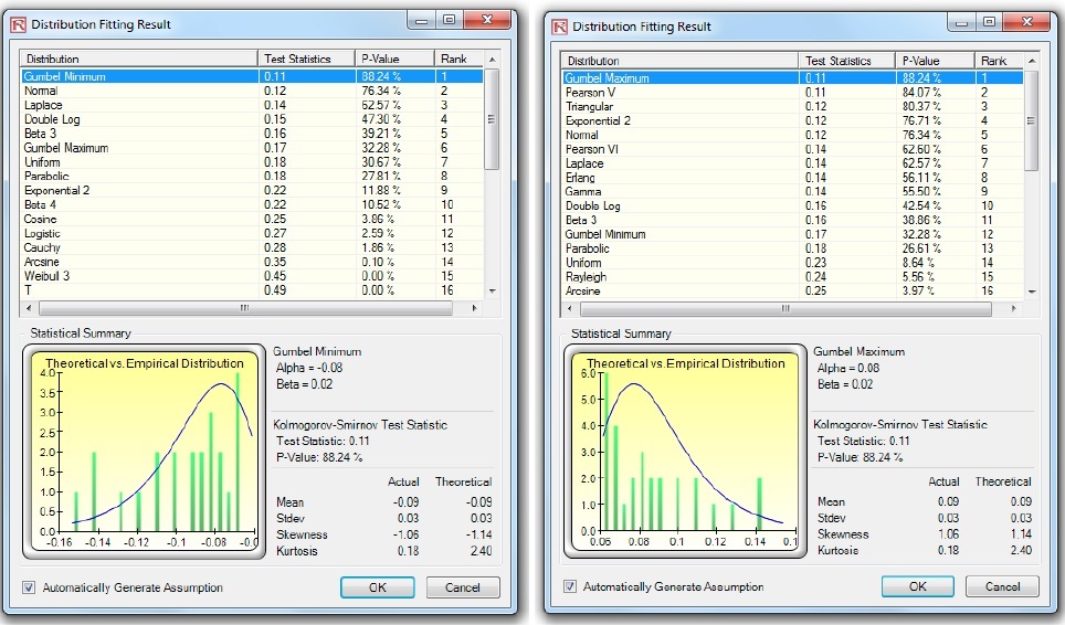
We see in Figure 5 that the negative losses fit the Gumbel Minimum Distribution the best, whereas the absolute positive losses fit the Gumbel Maximum Distribution the best. These two probability distributions are mirror images of each other and therefore using either distribution in your model would be fine. Figure 6 shows two additional sets of distributional fit on data with 4% and 7% loss thresholds, respectively. We see that the best-fitting dataset for the extreme value is at the 7% loss threshold (a higher p-value means a better fit, and a p-value of 93.71% on the 7% threshold data returns the best fit among the three).
We recommend using the Kolmogorov-Smirnov method as it is a nonparametric test and would be best suited for fitting extreme value tail events. You can also try the other fitting methods available in Risk Simulator’s BizStats module, including Anderson-Darling, Akaike Information Criterion, Schwartz/Bayes Criterion, Kuiper’s Statistics, and so forth.

To illustrate another method of data filtering, Figure 7 shows how a GARCH model can be run on the historical macroeconomic data. See the technical section later in this case study for the various GARCH model specifications (e.g., GARCH, GARCH-M, TGARCH, EGARCH, GJR-GARCH, etc.). In most situations, we recommend using either GARCH or EGARCH for extreme value situations. The generated GARCH volatility results can also be charted and we can visually inspect the periods of extreme fluctuations and refer back to the data to determine what those losses are. The volatilities can also be plotted as Control Charts in the Risk Simulator’s BizStats module (Figure 8) in order to determine at what point the volatilities are deemed statistically out of control, that is, extreme events.

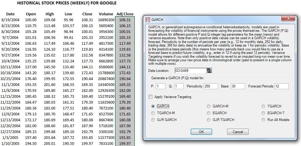
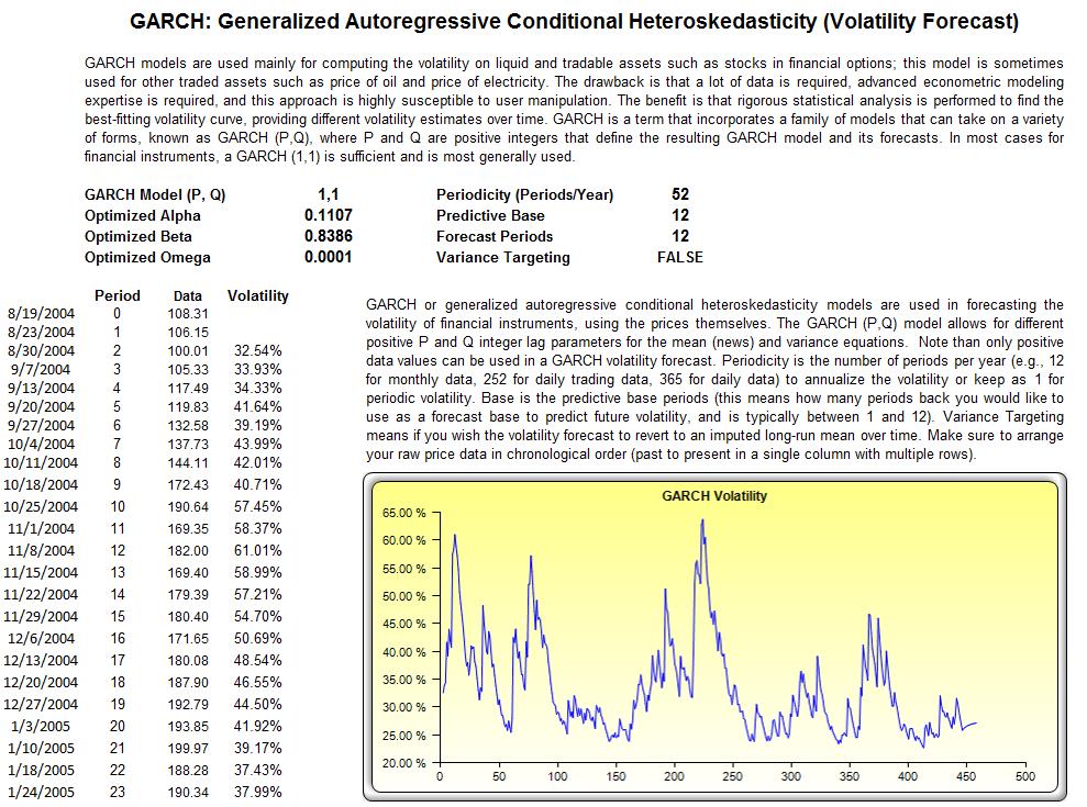
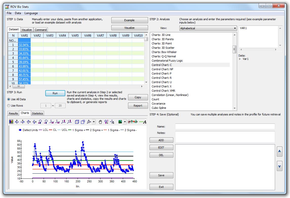
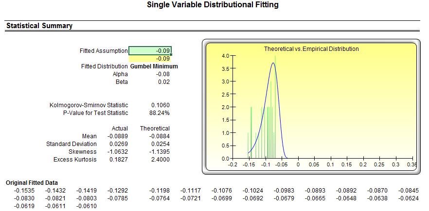
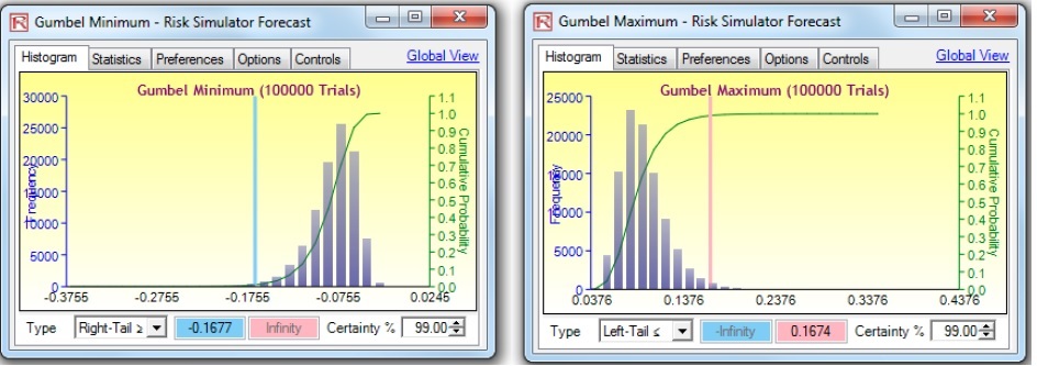
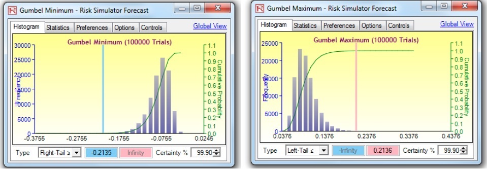
Figure 9 shows the distributional fitting report from Risk Simulator. If we run a simulation for 100,000 trials on both the Gumbel Minimum and Gumbel Maximum Distributions, we obtain the results shown in Figure 10. The VaR at 99% is computed to be a loss of –16.75% (averaged and rounded, taking into account both simulated distributions’ results). Compare this –16.75% value, which accounts for extreme shocks on the losses, to, say, the empirical historical value of a –11.62% loss (Figure 4), only accounting for a small window of actual historical returns, which may or may not include any extreme loss events. The VaR at 99.9% is computed as –21.35% (Figure 10).

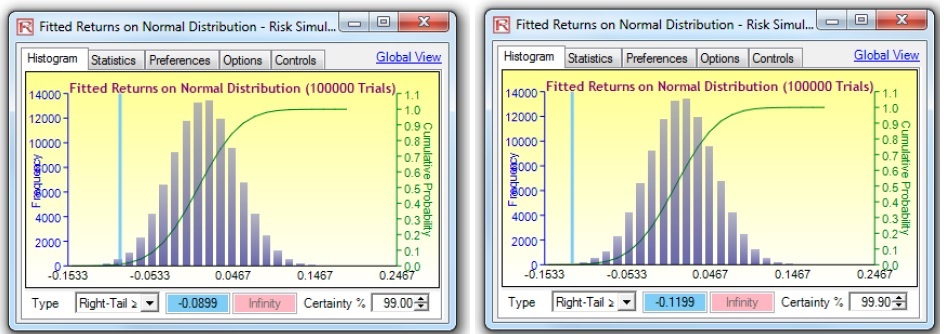
Further, as a comparison, if we assumed and used only a Normal Distribution to compute the VaR, the results would be significantly below what the extreme value stressed results should be. Figure 11 shows the results from the Normal Distribution VaR, where the 99% and 99.9% VaR show a loss of –8.99% and –11.99%, respectively, a far cry from the extreme values of –16.75% and –21.35%.

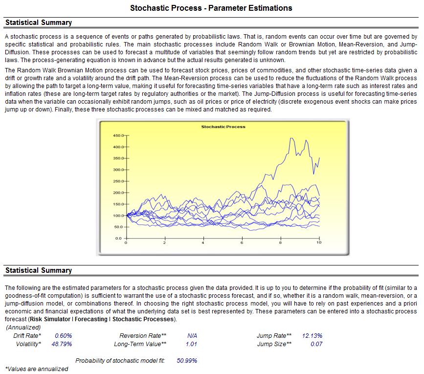
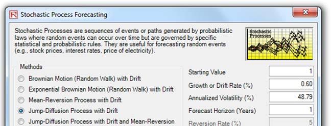
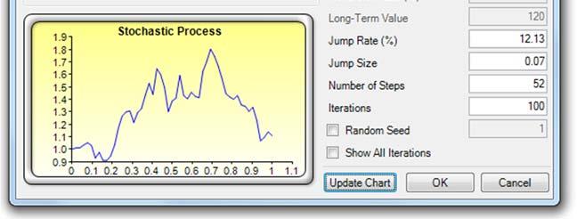
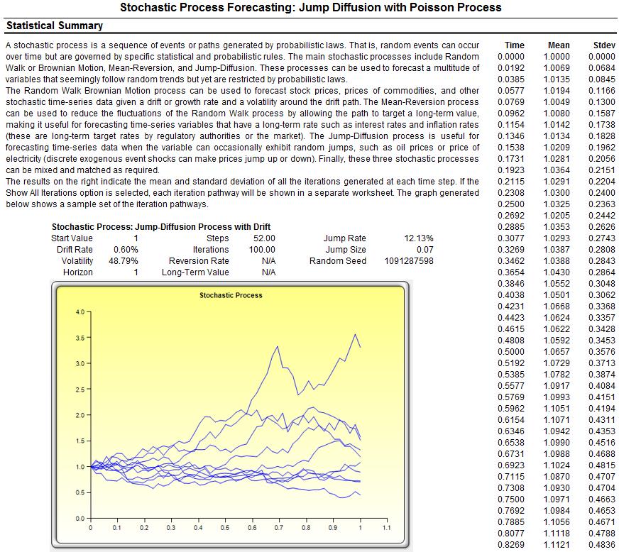
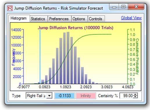
Another approach to predict, model, and stress test extreme value events is to use a Jump-Diffusion Stochastic Process with a Poisson Jump Probability. Such a model will require historical macroeconomic data to calibrate its inputs. For instance, using Risk Simulator’s Statistical Analysis module, the historical Google stock returns were subjected to various tests and the stochastic parameters were calibrated as seen in Figure 12. Stock returns were used as the first-differencing creates added stationarity to the data. The calibrated model has a 50.99% fit (small probabilities of fit are to be expected because we are dealing with real-life nonstationary data with high unpredictability). The inputs were then modeled in Risk Simulator | Forecast | Stochastic Processes module (Figure 13). The results generated by Risk Simulator are shown in Figure 14. As an example, if we use the end of Year 1’s results and set an assumption, in this case, a Normal Distribution with whatever mean and standard deviation is computed in the results report (Figure 14), a Monte Carlo risk simulation is run and the forecast results are shown in Figure 15, indicating that the VaR at 99% for this holding period is a loss of –11.33%. Notice that this result is consistent with Figure 4’s 1% percentile (left 1% is the same as right tail 99%) of –11.62%. In normal circumstances, this stochastic process approach is valid and sufficient, but when extreme values are to be analyzed for the purposes of extreme stress testing, the underlying requirement of a Normal Distribution in stochastic process forecasting would be insufficient in estimating and modeling these extreme shocks. And simply fitting and calibrating a stochastic process based only on extreme values would also not work as well as using, say, the Extreme Value Gumbel or Generalized Poisson Distributions.

 

 

Joint Dependence and T-Copula for Correlated Portfolios

Extreme co-movement of multiple variables occurs in the real world. For example, if the U.S. S&P500 index is down 25% today, we can be fairly confident that the Canadian market suffered a relatively large decline as well. If we modeled and simulated both market indices with a regular Normal copula to account for their correlations, this extreme comovement would not be adequately captured. The most extreme events for the individual indices in a Normal copula require that they be independent of each other (i.i.d. random). The T-copula, in contrast, includes a degrees-of-freedom input parameter to model the co-tendency for extreme events that can and do occur jointly. The T-copula enables the modeling of a co-dependency structure of the portfolio of multiple individual indices. The T-copula also allows for better modeling of fatter tails extreme events as opposed to the traditional assumption of jointly Normal portfolio returns of multiple variables.

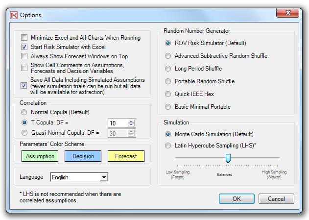
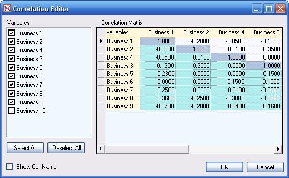
The approach to run such a model is fairly simple. Analyze each of the independent variables using the methods described above, and when these are inputted into a portfolio, compute the pairwise correlation coefficients, and then apply the T-copula in Risk Simulator available through the Risk Simulator | Options menu (Figure 16). The T-copula method employs a correlation matrix you enter, computes the correlation’s Cholesky-decomposed matrix on the inverse of the T Distribution, and simulates the random variable based on the selected distribution (e.g., Gumbel Max, Weibull 3, or Generalized Pareto Distribution).

Technical Details

Extreme Value Distribution or Gumbel Distribution

The Extreme Value Distribution (Type 1) is commonly used to describe the largest value of a response over a period of time, for example, in flood flows, rainfall, and earthquakes. Other applications include the breaking strengths of materials, construction design, and aircraft loads and tolerances. The Extreme Value Distribution is also known as the Gumbel Distribution.

The mathematical constructs for the Extreme Value Distribution are as follows:

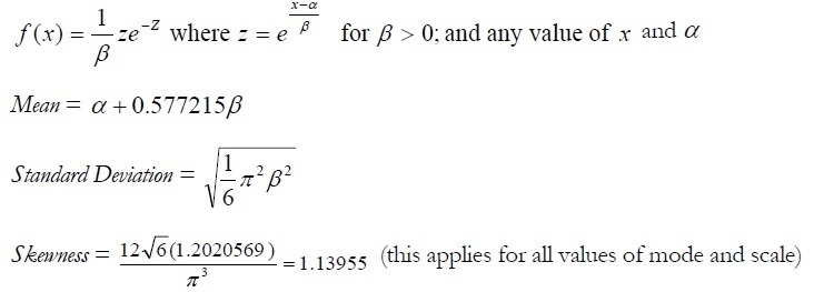
Excess Kurtosis = 5.4 (this applies for all values of mode and scale)
Mode (α) and scale (Β) are the distributional parameters.

Calculating Parameters
There are two standard parameters for the Extreme Value Distribution: mode and scale. The mode parameter is the most likely value for the variable (the highest point on the probability distribution). After you select the mode parameter, you can estimate the scale parameter. The scale parameter is a number greater than 0 .The larger the scale parameter, the greater the variance.

The Gumbel Maximum Distribution has a symmetrical counterpart, the Gumbel Minimum Distribution. Both are available in Risk Simulator. These two distributions are mirror images of each other where their respective  standard deviations and kurtosis are identical, but the Gumbel Maximum is skewed to the right (positive skew, with a higher probability on the left and lower probability on the right, as compared to the Gumbel Minimum, where the distribution is skewed to the left (negative skew). Their respective first moments are also mirror images of each other along the scale β parameter.

Input requirements:
Mode Alpha can be any value.
Scale Beta > 0.

 

 

 

 

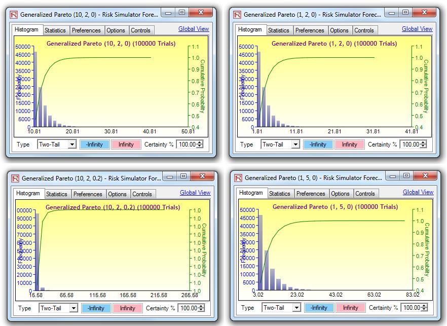
Generalized Pareto Distribution

The Generalized Pareto Distribution is often used to model the tails of another distribution.
The mathematical constructs for the Extreme Value Distribution are as follows:

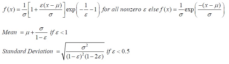
Location (µ), scale (Õ), and shape (ε) are the distributional parameters.
Input requirements:
Location Mu can be any value.
Scale Sigma > 0.

Shape Epsilon can be any value. ε < 0 would create a long-tailed distribution with no upper limit, whereas ε > 0 would generate a short-tailed distribution with a smaller variance and thicker right tail, where µ ≤ x < ∞. If Shape Epsilon and Location Mu are both zero, then the distribution reverts to the Exponential Distribution. If the Shape Epsilon is positive and Location Mu is exactly the ratio of Scale Sigma to Shape Epsilon, we have the regular ParetoDistribution. The Location Mu is sometimes also known as the threshold parameter.

Distributions whose tails decrease exponentially, such as the Normal Distribution, lead to a Generalized Pareto Distribution’s Shape Epsilon parameter of zero. Distributions whose tails decrease as a polynomial, such as Student’s T Distribution, lead to a positive Shape Epsilon parameter. Finally, distributions whose tails are finite, such as the Beta Distribution, lead to a negative Shape Epsilon parameter.

Weibull Distribution (Rayleigh Distribution)

The Weibull distribution describes data resulting from life and fatigue tests. It is commonly used to describe failure time in reliability studies as well as the breaking strengths of materials in reliability and quality control tests. Weibull Distributions are also used to represent various physical quantities, such as wind speed.

The Weibull Distribution is a family of distributions that can assume the properties of several other distributions.For example, depending on the shape parameter you define, the Weibull Distribution can be used to model the Exponential and Rayleigh Distributions, among others. The Weibull Distribution is very flexible. When the Weibull shape parameter is equal to 1.0, the Weibull Distribution is identical to the Exponential Distribution. The Weibull location parameter lets you set up an Exponential Distribution to start at a location other than 0.0. When the shape parameter is less than 1.0, the Weibull Distribution becomes a steeply declining curve. A manufacturer might find this effect useful in describing part failures during a burn-in period.
The mathematical constructs for the Weibull Distribution are as follows:

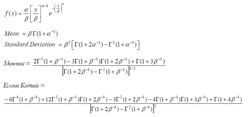
Shape (α) and central location scale (β) are the distributional parameters, and Γ is the Gamma function. Input requirements:
Shape Alpha ≥ 0.05.
Scale Beta > 0 and can be any positive value.
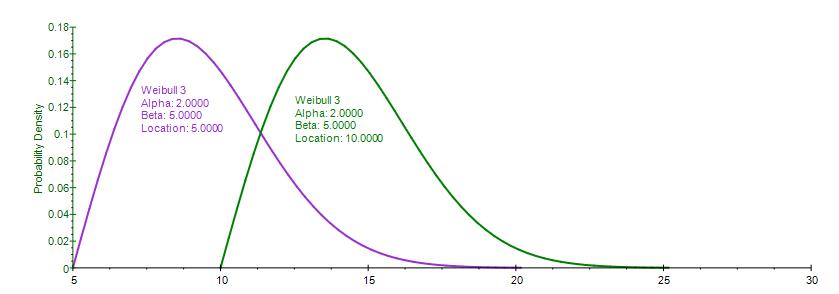
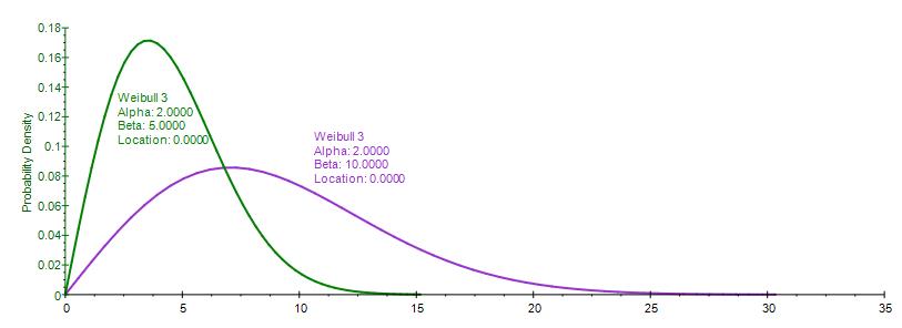
The Weibull 3 Distribution uses the same constructs as the original Weibull Distribution but adds a Location, or Shift, parameter. The Weibull Distribution starts from a minimum value of 0, whereas this Weibull 3, or Shifted Weibull, Distribution shifts the starting location to any other value.
Alpha, Beta, and Location or Shift are the distributional parameters.
Input requirements:
Alpha (Shape) ≥ 0.05.
Beta (Central Location Scale) > 0 and can be any positive value. Location can be any positive or negative value including zero.

 

GARCH Model: Generalized Autoregressive Conditional Heteroskedasticity
The generalized autoregressive conditional heteroskedasticity (GARCH) model is used to model historical and forecast future volatility levels of a marketable security (e.g., stock prices, commodity prices, oil prices, etc.). The dataset has to be a time series of raw price levels. GARCH will first convert the prices into relative returns and then run an internal optimization to fit the historical data to a mean-reverting volatility term structure, while assuming that the volatility is heteroskedastic in nature (changes over time according to some econometric characteristics). The theoretical specifics of a GARCH model are outside the purview of this case study.
Procedure

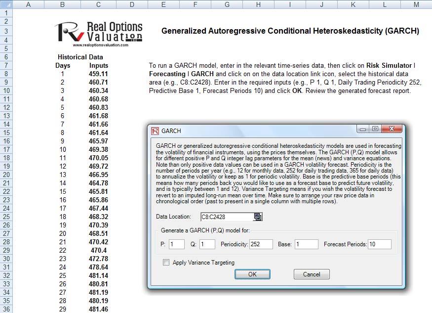
• Start Excel, open the example file Advanced Forecasting Model, go to the GARCH worksheet, and
  select Risk Simulator | Forecasting | GARCH.
• Click on the link icon, select the Data Location and enter the required input assumptions (see
  Figure 25), and click OK to run the model and report.

Notes

The typical volatility forecast situation requires P = 1, Q = 1; Periodicity = number of periods per year (12 for monthly data, 52 for weekly data, 252 or 365 for daily data); Base = minimum of 1 and up to the periodicity value; and Forecast Periods = number of annualized volatility forecasts you wish to obtain. There are several GARCH models available in Risk Simulator, including EGARCH, EGARCH-T, GARCH-M, GJR-GARCH, GJR-GARCH-T, IGARCH, and T-GARCH.

GARCH models are used mainly in analyzing financial time-series data to ascertain their conditional variances and volatilities. These volatilities are then used to value the options as usual, but the amount of historical data necessary for a good volatility estimate remains significant. Usually, several dozen––and even up to hundreds––of data points are required to obtain good GARCH estimates. GARCH is a term that incorporates a family of models that can take on a variety of forms, known as GARCH(p,q), where p and q are positive integers that define the resulting GARCH model and its forecasts. In most cases for financial instruments, a GARCH(1,1) is sufficient and is most generally used. For instance, a GARCH (1,1) model takes the form of:

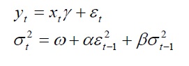
where the first equation’s dependent variable (yt) is a function of exogenous variables (xt) with an error term ( εt). The second equation estimates the variance (squared volatility σt²) at time t, which depends on a historical mean (ω), newsabout volatility from the previous period, measured as a lag of the squared residual from the mean equation (εt+1²), and volatility from the previous period (σt+1²). The exact modeling specification of a GARCH model is beyond the scopeof this case study. Suffice it to say that detailed knowledge of econometric modeling (model specification tests,structural breaks, and error estimation) is required to run a GARCH model, making it less accessible to the generalanalyst. Another problem with GARCH models is that the model usually does not provide a good statistical fit. That is, it is impossible to predict the stock market and, of course, equally if not harder to predict a stock’s volatility over time. Note that the GARCH function has several inputs as follow:

• Time-Series Data. The time series of data in chronological order (e.g., stock prices). Typically, dozens of data points are required for a decent volatility forecast.
• Periodicity. A positive integer indicating the number of periods per year (e.g., 12 for monthly data, 252 for daily trading data, etc.), assuming you wish to annualize the volatility. For getting periodic volatility, enter 1.
• Predictive Base. The number of periods back (of the time-series data) to use as a base to forecast volatility. The higher this number, the longer the historical base is used to forecast future volatility.
• Forecast Period. A positive integer indicating how many future periods beyond the historical stock prices you wish to forecast.
• Variance Targeting. This variable is set as False by default (even if you do not enter anything here) but can be set as True. False means the omega variable is automatically optimized and computed.The suggestion is to leave this variable empty. If you wish to create mean-reverting volatility with variance targeting, set this variable as True.
• P. The number of previous lags on the mean equation.
• Q. The number of previous lags on the variance equation.

The accompanying table lists some of the GARCH specifications used in Risk Simulator with two underlying distributional assumptions: one for Normal Distribution and the other for the T Distribution.

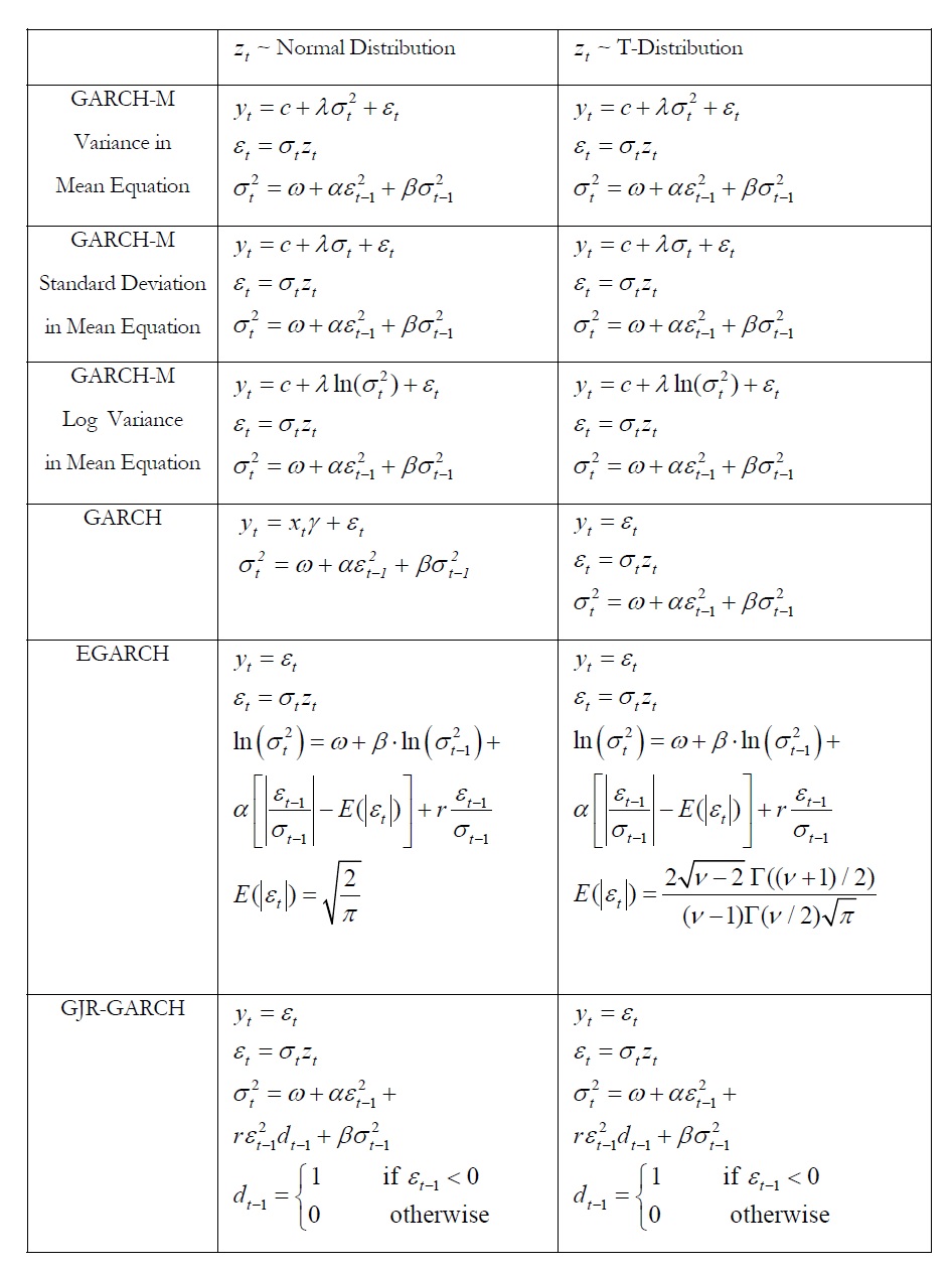
For the GARCH-M models, the conditional variance equations are the same in the six variations but the mean questions are different and assumption on zt can be either Normal Distribution or T Distribution. The estimated parameters for GARCH-M with Normal Distribution are those five parameters in the mean and conditional variance equations. The estimated parameters for GARCH-M with the T Distribution are those five parameters in the mean and conditional variance equations plus another parameter, the degrees of freedom for the T Distribution. In contrast, for the GJR models, the mean equations are the same in the six variations and the differences are that the conditional variance equations and the assumption on t z can be either a Normal Distribution or T Distribution. The estimated parameters for EGARCH and GJR-GARCH with Normal Distribution are those four parameters in the conditional variance equation. The estimated parameters for GARCH, EARCH, and GJR-GARCH with T Distribution are those parameters in the conditional variance equation plus the degrees of freedom for the T Distribution.

Economic Capital and Value at Risk Illustrations

Structural VaR Models

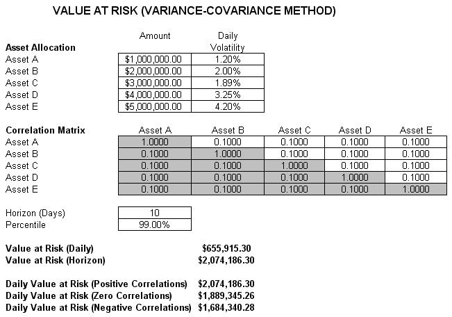
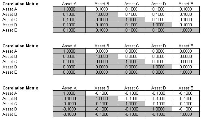
The first VaR example model shown is the Value at Risk – Static Covariance Method, accessible through Modeling Toolkit | Value at Risk | Static Covariance Method. This model is used to compute the portfolio’s VaR at a given percentile for a specific holding period, after accounting for the cross-correlation effects between the assets (Figure 26). The daily volatility is the annualized volatility divided by the square root of trading days per year. Typically, positive correlations tend to carry a higher VaR compared to zero correlation asset mixes, whereas negative correlations reduce the total risk of the portfolio through the diversification effect (Figures 26 and 27). The approach used is a portfolio VaR with correlated inputs, where the portfolio has multiple asset holdings with different amounts and volatilities. Assets are also correlated to each other. The covariance or correlation structural model is used to compute the VaR given a holding period or horizon and percentile value (typically 10 days at 99% confidence). Of course, the example illustrates only a few assets or business or credit lines for simplicity’s sake. Nonetheless, using the VaR functions in Modeling Toolkit (B2VaRCorrelationMethod), many more lines, asset, or businesses can be modeled.

VaR Models Using Monte Carlo Risk Simulation

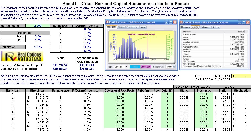
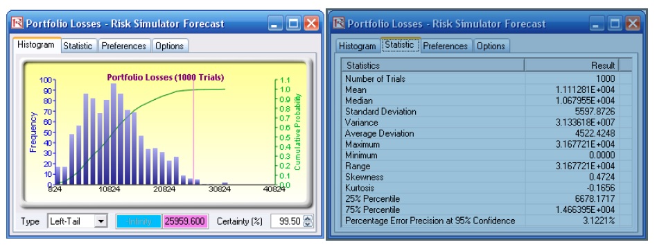
The model used is Value at Risk – Portfolio Operational and Capital Adequacy and is accessible through Modeling Toolkit | Value at Risk | Portfolio Operational and Capital Adequacy. This model shows how operational risk and credit risk parameters are fitted to statistical distributions and shows their resulting distributions are modeled in a portfolio of liabilities to determine the Value at Risk (99.50th percentile certainty) for the capital requirement under Basel II requirements. It is assumed that the historical data of the operational risk impacts (Historical Data worksheet) are obtained through econometric modeling of the Key Risk Indicators.

The Distributional Fitting Report worksheet is a result of running a distributional fitting routine in Risk Simulator to obtain the appropriate distribution for the operational risk parameters. Using the resulting distributional parameter,we model each liability’s capital requirements within an entire portfolio. Correlations can also be inputted, if required,between pairs of liabilities or business units. The resulting Monte Carlo simulation results show the Value at Risk, or VaR, capital requirements.

 

Note that an appropriate empirically based historical VaR cannot be obtained if distributional fitting and riskbased simulations were not first run. The VaR will be obtained only by running simulations. To perform distributional fitting, follow the steps below:

• In the Historical Data worksheet (Figure 28), select the data area (cells C5:L104) and click on Risk Simulator | Tools | Distributional Fitting (Single Variable).
• Browse through the fitted distributions and select the best-fitting distribution (in this case, the exponential distribution in Figure 29) and click OK.

 

 

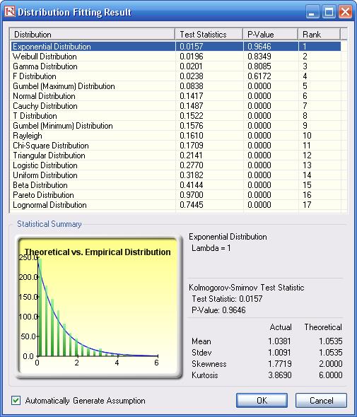
• You may now set the assumptions on the Operational Risk Factors with the Exponential Distribution (fitted results show Lambda = 1) in the Credit Risk worksheet. Note that the assumptions have already been set for you in advance. You may set the assumption by going to cell F27 and clicking on Risk Simulator | Set Input Assumption, selecting Exponential Distribution and entering 1 for the Lambda value and clicking OK. Continue this process for the remaining cells in column F, or simply perform a Risk Simulator Copy and Risk Simulator Paste on the remaining cells:
  • Note that since the cells in column F have assumptions set, you will first have to clear them if you wish
    to reset and copy/paste parameters. You can do so by first selecting cells F28:F126 and clicking on the
    Remove Parameter icon or select Risk Simulator | Remove Parameter.
  • Then select cell F27, click on the Risk Simulator Copy icon or select Risk Simulator | Copy Parameter, and then select cells F28:F126 and click on the Risk Simulator Paste icon or select Risk Simulator | Paste Parameter.
• Next, you can set additional assumptions, such as the probability of default using the Bernoulli Distribution(column H) and Loss Given Default (column J). Repeat the procedure in Step 3 if you wish to reset the assumptions.
• Run the simulation by clicking on the Run icon or clicking on Risk Simulator | Run Simulation.
• Obtain the Value at Risk by going to the forecast chart once the simulation is done running and selecting Left-Tail and typing in 99.50. Hit Tab on the keyboard to enter the confidence value and obtain the VaR of $25,959 (Figure 30).

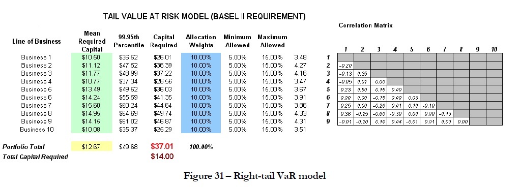
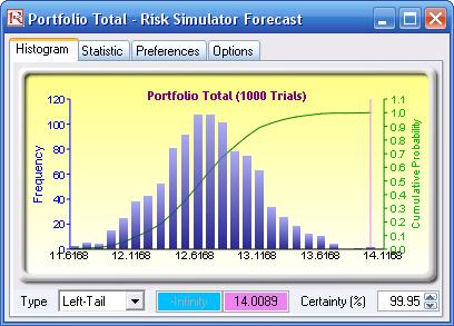
Another example on VaR computation is shown next, where the model Value at Risk – Right Tail Capital Requirements is used, available through Modeling Toolkit | Value at Risk | Right Tail Capital Requirements. This model shows the capital requirements per Basel II requirements (99.95th percentile capital adequacy based on a specific holding period’s Value at Risk). Without running risk-based historical and Monte Carlo simulation using Risk Simulator, the required capital is $37.01M (Figure 31) as compared to only $14.00M that is required using a correlated simulation (Figure 32). This is due to the cross-correlations between assets and business lines, and can be modeled only using Risk Simulator. This lower VaR is preferred as banks can now be required to hold less required capital and can reinvest the remaining capital in various profitable ventures, thereby generating higher profits.

 

• To run the model, click on Risk Simulator | Run Simulation (if you had other models open, make sure you first click on Risk Simulator | Change Simulation | Profile, and select the Tail VaR profile before starting).
• When the simulation run is complete, select Left-Tail in the forecast chart and enter in 99.95 in the Certainty box and hit TAB on the keyboard to obtain the value of $14.00M Value at Risk for this correlated simulation.
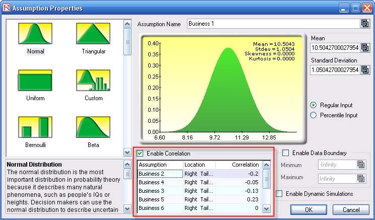
• Note that the assumptions have already been set for you in advance in the model in cells C6:C15. However,you may set them again by going to cell C6 and clicking on Risk Simulator | Set Input Assumption, selecting yourdistribution of choice or using the default Normal Distribution or performing a distributional fitting onhistorical data, then clicking OK. Continue this process for the remaining cells in column C. You may also decide to first Remove Parameters of these cells in column C and then set your own distributions. Further,
  correlations can be set manually when assumptions are set (Figure 31) or by going to Risk Simulator | Edit
  Correlations (Figure 32) after all the assumptions are set.

 

 

If risk simulation was not run, the VaR or economic capital required would have been $37M, as opposed to only $14M. All cross-correlations between business lines have been modeled, as are stress and scenario tests, and thousands and thousands of possible iterations are run. Individual risks are now aggregated into a cumulative portfolio level VaR.

Efficient Portfolio Allocation and Economic Capital VaR

As a side note, by performing portfolio optimization, a portfolio’s VaR actually can be reduced. We start by first introducing the concept of stochastic portfolio optimization through an illustrative hands-on example. Then, using this portfolio optimization technique, we apply it to four business lines or assets to compute the VaR or an un-optimized versus an optimized portfolio of assets, and see the difference in computed VaR. You will note that at the end, the optimized portfolio bears less risk and has a lower required economic capital.

Stochastic Portfolio Optimization

The optimization model used to illustrate the concepts of stochastic portfolio optimization is Optimization – Stochastic Portfolio Allocation and it can be accessed via Modeling Toolkit | Optimization | Stochastic Portfolio Allocation. This model shows four asset classes with different risk and return characteristics. The idea here is to find the best portfolio allocation such that the portfolio’s bang for the buck or returns to risk ratio is maximized. That is, in order to allocate 100% of an individual’s investment among several different asset classes (e.g., different types of mutual funds or investment styles: growth, value, aggressive growth, income, global, index, contrarian, momentum, and so forth), optimization is used. This model is different from others in that there exist several simulation assumptions (risk and return values for each asset), as seen in Figure 35. That is, a simulation is run, then optimization is executed, and the entire process is repeated multiple times to obtain distributions of each decision variable. The entire analysis can be automated using Stochastic Optimization

In order to run an optimization, several key specifications on the model have to first be identified:

• Objective: Maximize Return to Risk Ratio (C12)
• Decision Variables: Allocation Weights (E6:E9)
• Restrictions on Decision Variables: Minimum and Maximum Required (F6:G9).
• Constraints: Portfolio Total Allocation Weights 100% (E11 is set to 100%)
• Simulation Assumptions: Return and Risk Values (C6:D9)

The model shows the various asset classes. Each asset class has its own set of annualized returns and annualized volatilities. These return and risk measures are annualized values such that they can be compared consistently across different asset classes. Returns are computed using the geometric average of the relative returns, while the risks are computed using the logarithmic relative stock returns approach.

Column E, Allocation Weights, holds the decision variables, which are the variables that need to be tweaked and tested such that the total weight is constrained at 100% (cell E11). Typically, to start the optimization, we will set these cells to a uniform value, where in this case, cells E6 to E9 are set at 25% each. In addition, each decision variable may have specific restrictions in its allowed range. In this example, the lower and upper allocations allowed are 10% and 40%, as seen in columns F and G. This setting means that each asset class can have its own allocation boundaries.

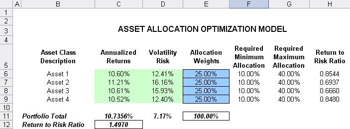
Next, column H shows the Return to Risk Ratio, which is simply the return percentage divided by the risk percentage, where the higher this value, the higher the bang for the buck. The remaining sections of the model show the individual asset class rankings by returns, risk, return to risk ratio, and allocation. In other words, these rankings show at a glance which asset class has the lowest risk, or the highest return, and so forth.

Running an Optimization

To run this model, simply click on Risk Simulator | Optimization | Run Optimization. Alternatively, and for practice, you can set up the model using the following approach:

• Start a new profile (Risk Simulator | New Profile).
• For stochastic optimization, set distributional assumptions on the risk and returns for each asset class. That is, select cell C6 and set an assumption (Risk Simulator | Set Input Assumption) and make your own assumption as required. Repeat for cells C7 to D9
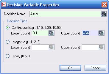
• Select cell E6, and define the decision variable (Risk Simulator | Optimization | Decision Variables or click on the Define Decision icon) and make it a Continuous Variable and then link the decision variable’s name and minimum/maximum required to the relevant cells (B6, F6, G6).
• Then use the Risk Simulator Copy on cell E6, select cells E7 to E9, and use Risk Simulator’s Copy (Risk Simulator | Copy Parameter) and Risk Simulator | Paste Parameter, or use the copy and paste icons.
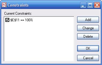
• Next, set up the optimization’s constraints by selecting Risk Simulator | Optimization | Constraints, selecting ADD, and selecting the cell E11, and making it equal 100% (total allocation, and do not forget the % sign).
• Select cell C12, the objective to be maximized and make it the objective: Risk Simulator | Optimization | Set Objective or click on the O icon.
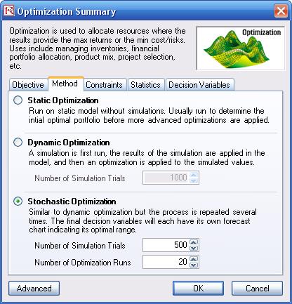
• Run the simulation by going to Risk Simulator | Optimization | Run Optimization. Review the different tabs to make sure that all the required inputs in steps 2 and 3 above are correct. Select Stochastic Optimization and let it run for 500 trials repeated 20 times (Figure 36 illustrates these setup steps).

You may also try other optimization routines where:

Discrete Optimization is an optimization that is run on a discrete or static model, where no simulations are run. This optimization type is applicable when the model is assumed to be known and no uncertainties exist. Also, a discrete optimization can be run first to determine the optimal portfolio and its corresponding optimal allocation of decision variables before more advanced optimization procedures are applied. For instance, before running a stochastic optimization problem, a discrete optimization is run first to determine if there exist solutions to the optimization problem before a more protracted analysis is performed.

Dynamic Optimization is applied when Monte Carlo simulation is used together with optimization. Another name for such a procedure is Simulation-Optimization. In other words, a simulation is run for N trials, and then an optimization process is run for M iterations until the optimal results are obtained or an infeasible set is found. That is, using Risk Simulator’s optimization module, you can choose which forecast and assumption statistics to use and replace in the model after the simulation is run. Then, these forecast statistics
can be applied in the optimization process. This approach is useful when you have a large model with many interacting assumptions and forecasts, and when some of the forecast statistics are required in the optimization.

Stochastic Optimization is similar to the dynamic optimization procedure except that the entire dynamic optimization process is repeated T times. The results will be a forecast chart of each decision variable with T values. In other words, a simulation is run and the forecast or assumption statistics are used in the optimization model to find the optimal allocation of decision variables. Then another simulation is run, generating different forecast statistics, and these new updated values are then optimized, and so forth. Hence, each of the final decision variables will have its own forecast chart, indicating the range of the optimal decision variables. For instance, instead of obtaining single-point estimates in the dynamic optimization procedure, you can now obtain a distribution of the decision variables, and, hence, a range of optimal values for each decision variable, also known as a stochastic optimization.

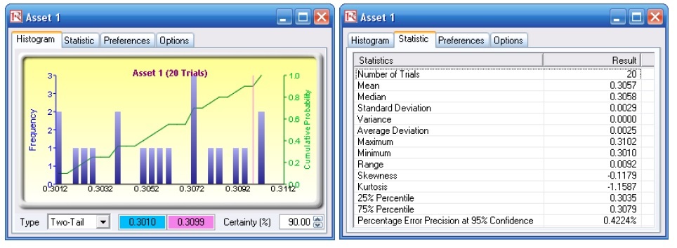
Viewing and Interpreting Forecast Results Stochastic optimization is performed when a simulation is first run and then the optimization is run. Then the whole analysis is repeated multiple times. The result is a distribution of each decision variable, rather than a single point estimate (Figure 37). This distribution means that instead of saying you should invest 30.57% in Asset 1, the optimal decision is to invest between 30.10% and 30.99% as long as the total portfolio sums to 100%. This way, the optimization results provide management or decision makers a range of flexibility in the optimal decisions. Refer to Chapter 11 of Modeling Risk: Applying Monte Carlo Simulation, Real Options Analysis, Forecasting, and Optimization by Dr. Johnathan Mun for more detailed explanations about this model and the different optimization techniques, as well as an interpretation of the results. Chapter 11’s appendix also details how the risk and return values are computed.

Portfolio Optimization and Portfolio VaR Now that we understand the concepts of optimized portfolios, let us see what the effects are on computed economic capital through the use of a correlated portfolio VaR. This model uses Monte Carlo simulation and optimization
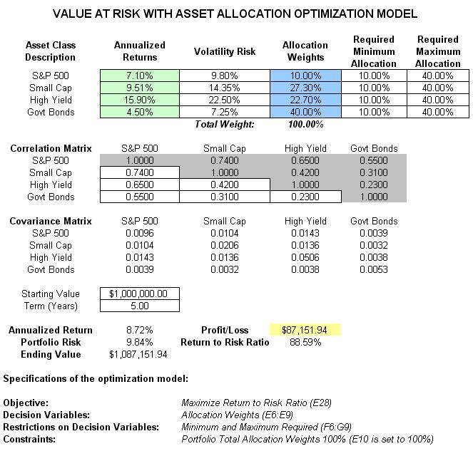
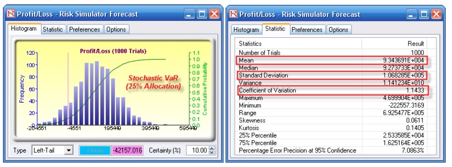
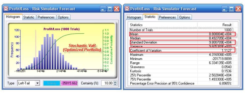
routines in Risk Simulator to minimize the VaR of a portfolio of assets (Figure 38). The file used is Value at Risk – Optimized and Simulated Portfolio VaR, which is accessible via Modeling Toolkit | Value at Risk | Optimized and Simulated Portfolio VaR. In this example, we intentionally used only 4 asset classes to illustrate the effects of an optimized portfolio. In real life, we can extend this process to cover a multitude of asset classes and business lines. Here, we now illustrate the use of a left-tail VaR as opposed to a right-tail VaR, but the concepts are similar. First, simulation is used to determine the 90% left-tail VaR. The 90% left-tail probability means that there is a 10% chance that losses will exceed this VaR for a specified holding period. With an equal allocation of 25% across the 4 asset classes, the VaR is determined using simulation (Figure 39). The annualized returns are uncertain and hence simulated. The VaR is then read off the forecast chart. Then, optimization is run to find the best portfolio subject to the 100% allocation across the 4 projects that will maximize the portfolio’s bang for the buck (returns to risk ratio). The resulting optimized portfolio is then simulated once again and the new VaR is obtained (Figure 40). The VaR of this optimized portfolio is a lot less than the not optimized portfolio. That is, the expected loss is $35.8M instead of $42.2M, which means that the bank will have a lower required economic capital if the portfolio of holdings is first optimized.

< br />