Box-Jenkins ARIMA Advanced Time Series

• By Admin
• November 19, 2014
• Comments Off on Box-Jenkins ARIMA Advanced Time Series

Theory
One very powerful advanced times-series forecasting tool is the ARIMA or Auto-Regressive Integrated Moving Average approach, which assembles three separate tools into a comprehensive model. The first tool segment is the autoregressive or “AR” term, which corresponds to the number of lagged value of the residual in the unconditional forecast model. In essence, the model captures the historical variation of actual data to a forecasting model and uses this variation or residual to create a better predicting model. The second tool segment is the integration order or the “I” term. This integration term corresponds to the number of differencing the time series to be forecasted goes through to make the data stationary. This element accounts for any nonlinear growth rates existing in the data. The third tool segment is the moving average or “MA” term, which is essentially the moving average of lagged forecast errors. By incorporating this lagged forecast errors component, the model in essence learns from its forecast errors or mistakes and corrects for them through a moving average calculation.

The ARIMA model follows the Box-Jenkins methodology with each term representing steps taken in the model construction until only random noise remains. Also, ARIMA modeling uses correlation techniques in generating forecasts. ARIMA can be used to model patterns that may not be visible in plotted data. In addition, ARIMA models can be mixed with exogenous variables, but you must make sure that the exogenous variables have enough data points to cover the additional number of periods to forecast. Finally, be aware that ARIMA cannot and should not be used to forecast stochastic processes or time-series data that are stochastic in nature––use the Stochastic Process module to forecast instead.

There are many reasons why an ARIMA model is superior to common time-series analysis and multivariate regressions. The usual finding in time-series analysis and multivariate regression is that the error residuals are correlated with their own lagged values. This serial correlation violates the standard assumption of regression theory that disturbances are not correlated with other disturbances. The primary problems associated with serial correlation are:

• Regression analysis and basic time-series analysis are no longer efficient among the different linear estimators. However, as the error residuals can help to predict current error residuals, we can take advantage of this information to form a better prediction of the dependent variable using ARIMA.
• Standard errors computed using the regression and time-series formula are not correct and are generally understated. If there are lagged dependent variables set as the regressors, regression estimates are biased and inconsistent but can be fixed using ARIMA.

Autoregressive Integrated Moving Average, or ARIMA(p,d,q), models are the extension of the AR model that uses three components for modeling the serial correlation in the timeseries data. As previously noted, the first component is the autoregressive (AR) term. The AR(p) model uses the p lags of the time series in the equation. An AR(p) model has the form: yt = a1yt-1 + … + apyt-p + et. The second component is the integration (d) order term. Each integration order corresponds to differencing the time series. I(1) means differencing the data once; I(d) means differencing the data d times. The third component is the moving average (MA) term. The MA(q) model uses the q lags of the forecast errors to improve the forecast. An MA(q) model has the form: yt = et + b1et-1 + … + bqet-q. Finally, an ARMA(p,q) model has the combined form: yt = a1 yt-1 + … + a p yt-p + et + b1 et-1 + … + bq et-q.

Procedure

• Start Excel and enter your data or open an existing worksheet with historical data to forecast (Figure 1 uses the example file Time-Series Forecasting).
• Click on Risk Simulator | Forecasting | ARIMA and select the time-series data.
• Enter the relevant p, d, and q parameters (positive integers only) and enter the number of forecast periods desired, and click OK.

Results Interpretation
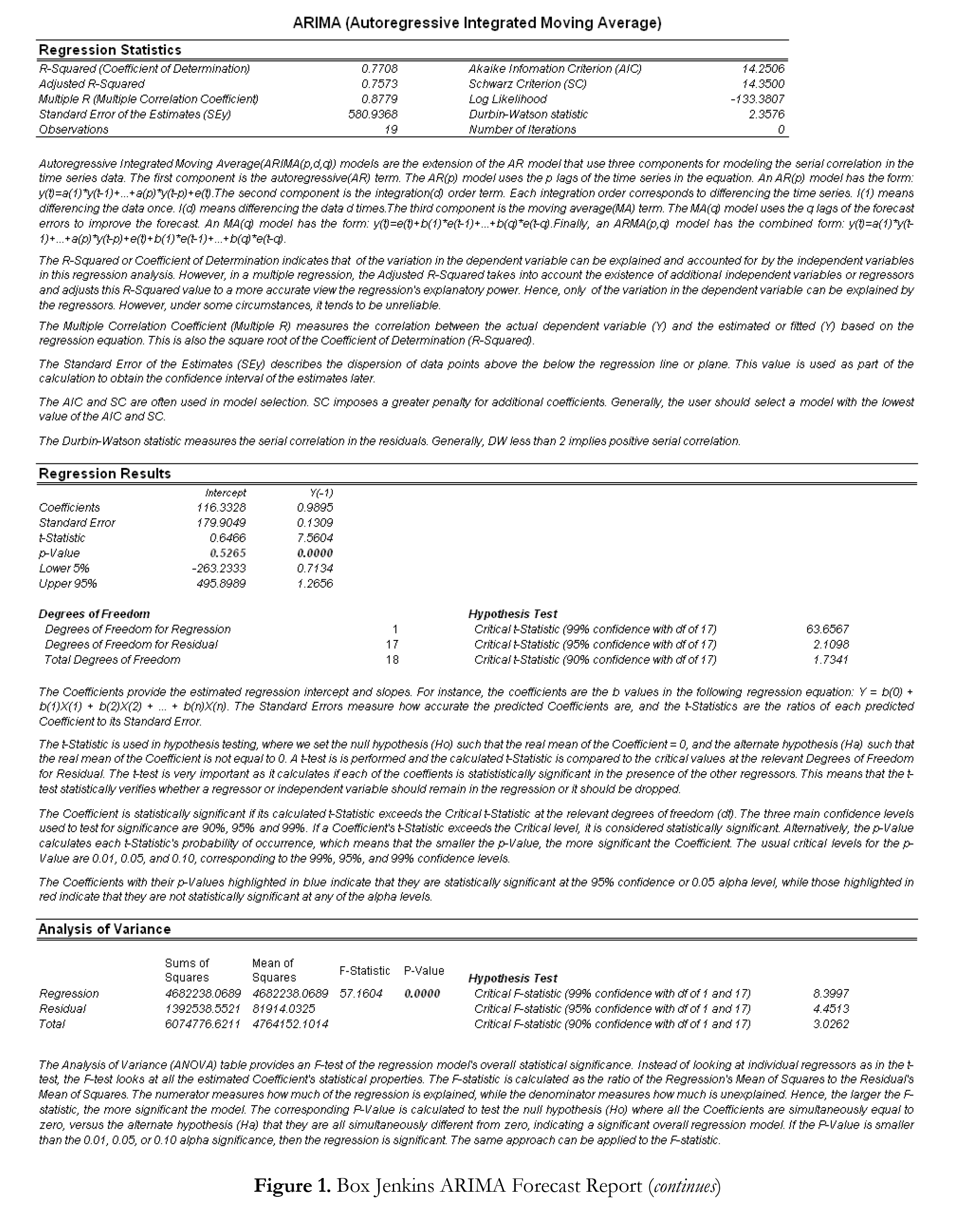
In interpreting the results of an ARIMA model, most of the specifications are identical to the multivariate regression analysis (see Chapter 9, Using the Past to Predict the Future, in Modeling Risk, Second Edition, for more technical details about interpreting the multivariate regression analysis and ARIMA models). However, there are several additional sets of results specific to the ARIMA analysis as seen in Figure 1. The first is the addition of Akaike Information Criterion (AIC) and Schwarz Criterion (SC), which are often used in ARIMA model selection and identification. That is, AIC and SC are used to determine if a particular model with a specific set of p, d, and q parameters is a good statistical fit. SC imposes a greater penalty for additional coefficients than the AIC, but generally the model with the lowest AIC and SC values should be chosen. Finally, an additional set of results called the autocorrelation (AC) and partial autocorrelation (PAC) statistics are provided in the ARIMA report.

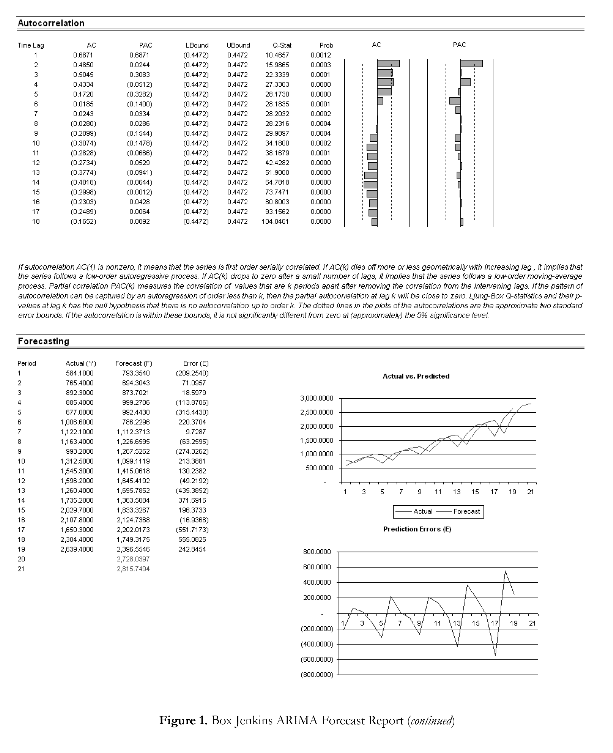
For instance, if autocorrelation AC(1) is nonzero, it means that the series is first-order serially correlated. If AC dies off more or less geometrically with increasing lags, it implies that the series follows a low-order autoregressive process. If AC drops to zero after a small number of lags, it implies that the series follows a low-order moving-average process. In contrast, PAC measures the correlation of values that are k periods apart after removing the correlation from the intervening lags. If the pattern of autocorrelation can be captured by an autoregression of order less than k, then the partial autocorrelation at lag k will be close to zero. The Ljung-Box Q-statistics and their p-values at lag k are also provided, where the null hypothesis being tested is such that there is no autocorrelation up to order k. The dotted lines in the plots of the autocorrelations are the approximate two standard error bounds. If the autocorrelation is within these bounds, it is not significantly different from zero at approximately the 5% significance level. Finding the right ARIMA model takes practice
and experience. These AC, PAC, SC, and AIC elements are highly useful diagnostic tools to help identify the correct model specification. Finally, the ARIMA parameter results are obtained using sophisticated optimization and iterative algorithms, which means that although the functional forms look like those of a multivariate regression, they are not the same. ARIMA is a much more computationally intensive and advanced econometric approach.

Auto ARIMA (Box–Jenkins ARIMA Advanced Time-Series)

Theory
This tool provides analyses identical to the ARIMA module except that the Auto-ARIMA module automates some of the
traditional ARIMA modeling by automatically testing multiple permutations of model specifications and returns the bestfitting model. Running the Auto-ARIMA module is similar to running regular ARIMA forecasts. The differences being that the p, d, q inputs are no longer required and that different combinations of these inputs are automatically run and compared.

Procedure

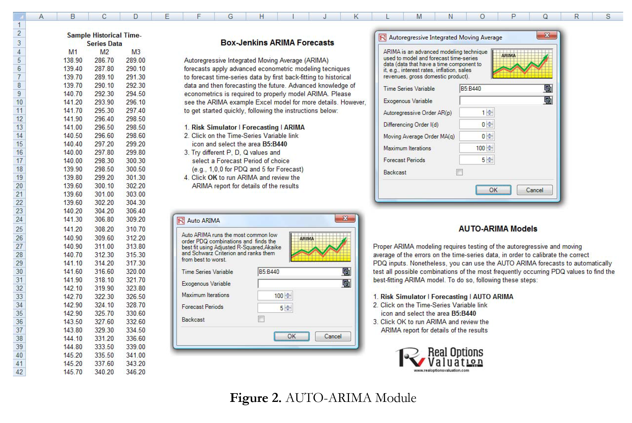
• Start Excel and enter your data or open an existing worksheet with historical data to forecast (the illustration shown in Figure 2 uses the example file Advanced Forecasting Models in the Examples menu of Risk Simulator).
• In the Auto ARIMA worksheet, select Risk Simulator | Forecasting | AUTO-ARIMA. You can also access the method through the Forecasting icons ribbon or right-clicking anywhere in the model and selecting the forecasting shortcut menu.
• Click on the link icon and link to the existing time-series data, enter the number of forecast periods desired, and click OK.

ARIMA and AUTO ARIMA Note
For ARIMA and Auto ARIMA, you can model and forecast future periods either by using only the dependent variable (Y), that is, the Time Series Variable by itself, or you can insert additional exogenous variables (X1, X2,…, Xn) just as in a regression analysis where you have multiple independent variables. You can run as many forecast periods as you wish if you only use the time-series variable (Y). However, if you add exogenous variables (X), be sure to note that your forecast periods are limited to the number of exogenous variables’ data periods minus the time-series variable’s data periods. For example, you can only forecast up to 5 periods if you have time-series historical data of 100 periods and only if you have exogenous variables of 105 periods (100 historical periods to match the time-series variable and 5 additional future periods of independent exogenous variables to forecast the time-series dependent variable).