Case Study: Basel II and Basel III Credit, Market, Operational, and Liquidity Risks with Asset Liability Management

• By Admin
• January 28, 2015
• Comments Off on Case Study: Basel II and Basel III Credit, Market, Operational, and Liquidity Risks with Asset Liability Management

This case study looks at the modeling and quantifying of Regulatory Capital, Key Risk Indicators,
Probability of Default, Exposure at Default, Loss Given Default, Liquidity Ratios, and Value at Risk, using
quantitative models, Monte Carlo risk simulations, credit models, and business statistics. It relates to the modeling and analysis of Asset Liability Management, Credit Risk, Market Risk, Operational Risk, and Liquidity Risk for banks or financial institutions, allowing these firms to properly identify, assess, quantify,value, diversify, hedge, and generate periodic regulatory reports for supervisory authorities and Central Banks on their credit, market, and operational risk areas, as well as for internal risk audits, risk controls,and risk management purposes.

In banking finance and financial services firms, economic capital is defined as the amount of risk capital, assessed on a realistic basis based on actual historical data, the bank or firm requires to cover the risks as a going concern, such as market risk, credit risk, liquidity risk, and operational risk. It is the amount of money that is needed to secure survival in a worst‐case scenario. Firms and financial services regulators such as Central Banks, Bank of International Settlements, and other regulatory commissions should then aim to hold an amount of risk capital equal at least to its economic capital.Typically,economic capital is calculated by determining the amount of capital that the firm needs to ensure that its realistic balance sheet stays solvent over a certain time period with a pre‐specified probability(e.g.,usually defined as 99.00%).Therefore, economic capital is often calculated as Value at Risk (VaR).

Figure 1 illustrates the PEAT utility’s ALM‐CMOL module for Credit Risk—Economic RegulatoryCapital’s (ERC) Global Settings tab. This current analysis is performed on credit issues such as loans, credit lines, and debt at the commercial, retail, or personal levels. To get started with the utility, existing files can be opened or saved, or a default sample model can be retrieved from the menu. The number of categories of loans and credit types can be set as well as the loan or credit category names, a loss given default (LGD) value in percent, and the Basel credit type (residential mortgages, revolving credit, other miscellaneous credit, or wholesale corporate and sovereign debt). Each credit type has its required Basel III model that is public knowledge, and the software uses the prescribed models per Basel regulations. Further, historical data can be manually entered by the user into the utility or via existing databases and data files.Such data files may be large and, hence, stored either in a single file or multiple data files where each file’s contents can be mapped to the list of required variables (e.g., credit issue date, customer information,product type or segment, Central Bank ratings, amount of the debt or loan, interest payment, principal payment, last payment date, and other ancillary information the bank or financial services firm has access to) for the analysis, and the successfully mapped connections are displayed. Additional information such as the required Value at Risk (VaR) percentiles, average life of a commercial loan, and historical data period on which to run the data files to obtain the probability of default (PD) are entered. Next, the Exposure at Default (EAD) analysis periodicity is selected as is the date type and the Central Bank ratings.Different Central Banks in different nations tend to have similar credit ratings but the software allows for flexibility in choosing the relevant rating scheme (i.e., Level 1 may indicate on‐time payment of an existing loan whereas Level 3 may indicate a late payment of over 90 days and, therefore, constitutes a default).All these inputs and settings can be saved either as stand‐alone settings and data or including the results.Users would enter a unique name and notes and Save the current settings(previously saved models and settings can be retrieved,Edited,or Deleted, a New model can be created,or an existing model can be
duplicated through a Save As).The saved models are listed and can be rearranged according to the user’s preference.

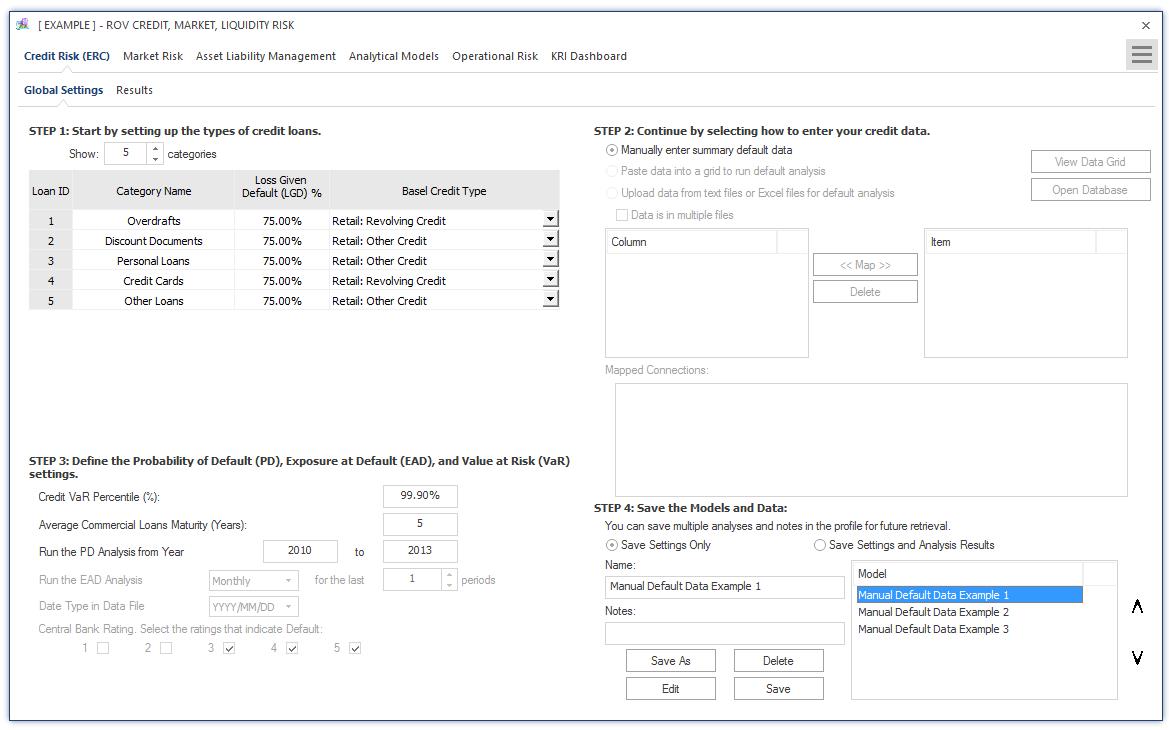
Figure 2 illustrates the PEAT utility’s ALM‐CMOL module for Credit Risk—Economic Regulatory Capital’s (ERC) Results tab. The results are shown in the grid if data files were loaded and preprocessed and results were computed and presented here (the loading of data files was discussed in connection with Figure 1, and the preprocessing of a bank’s data will be discussed in a later section). However, if data are to be manually entered (as previously presented in Figure 1), then the white areas in the data grid are available for manual user input, such as the number of clients for a specific credit or debt category, the number of defaults for said categories historically by period, and the exposure at default values (total amount of debt issued within the total period). One can manually input the number of clients and number of credit and loan defaults within specific annual time‐period bands. The utility computes the percentage of defaults (number of credit or loan defaults divided by number of clients within the specified time periods),and the average percentage of default is the proxy used for the Probability of Default (PD). If users have specific PD rates to use, they can simply enter any number of clients and number of defaults as long as the ratio is what the user wants as the PD input (e.g., a 1% PD means users can enter 100 clients and 1 as the number of default).The Loss Given Default (LGD) can be user inputted in the global settings as a percentage (LGD is defined as the percentage of losses of loans and debt that cannot be recovered when they are in default). The Exposure at Default (EAD) is the total loans amount within these time bands. These PD, LGD, and EAD values can also be computed using structural models as will be discussed later. Expected Losses (EL) is the product of PD × LGD × EAD.Economic Capital (EC) is based on Basel II and Basel III requirements and is a matter of public record. Risk Weighted Average (RWA) is a regulatory requirement per Basel II and Basel III such as 12.5 × EC. The change in Capital Adequacy Requirement (CAR @ 8%) is simply the ratio of the EC to EAD less the 8% holding requirement. In other words, the Regulatory Capital (RC) is 8% of EAD.

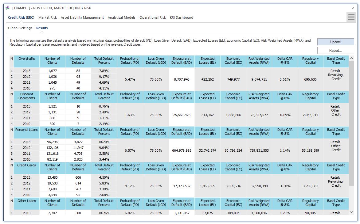
Figure 3 illustrates the PEAT utility’s ALM‐CMOL module for Market Risk where Market Data is entered. Users start by entering the global settings, such as the number of investment assets and currency assets the bank has in its portfolio, that require further analysis, the total number of historical data that will be used for analysis, and various Value at Risk percentiles to run (e.g., 99.00% and 95.00%). In addition, the volatility method of choice (industry standard volatility or Risk Metrics volatility methods) and the date type (mm/dd/yyyy or dd/mm/yyyy) are entered. The amount invested (balance) of each asset and currency is entered and the historical data can be entered, copy and pasted from another data source, or uploaded to the data grid, and the settings as well as the historical data entered can be saved for future retrieval and further analysis in subsequent subtabs.

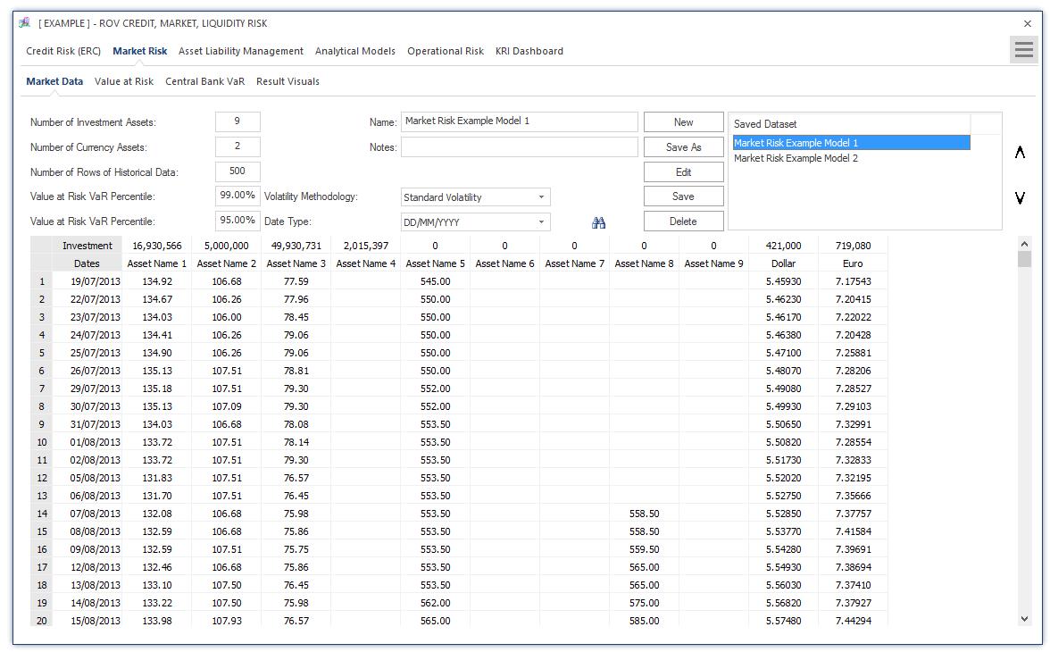
Figure 4 illustrates the computed results for the Market Value at Risk (VaR). Based on the data entered
in Figure 3’s interface, the results are computed and presented in two separate grids: the Value at Risk
(VaR) results and asset positions and details. The computations can be triggered to be rerun or Updated,
and the results can be exported to an Excel report template if required. The results computed in the first grid are based on user input market data. For instance, the Value at Risk (VaR) calculations are simply the Asset Position × Daily Volatility × Inverse Standard Normal Distribution of VaR Percentile × Square Root of the Horizon in Days.Therefore, the Gross VaR is simply the summation of all VaR values for all assets and foreign exchange denominated assets.In comparison, the Internal Historical Simulation VaR uses the same calculation based on historically simulated time‐series of asset values. The historically simulated time‐series of asset values is obtained by the Asset’s Investment × Asset Pricet‐1 × Period‐Specific Relative Returns – Asset’s Current Position. The Asset’s Current Position is simply the Investment × Asset Pricet. From this simulated time‐series of asset flows, the (1 – X%) percentile asset value is the VaR X%. Typically,X% is 99.00% or 95.00% and can be changed as required by the user based on the regional or country‐specific regulatory agency’s statutes.

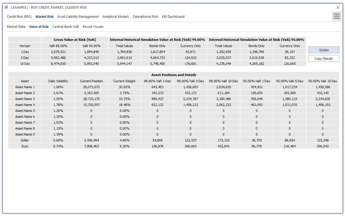
Figure 5 illustrates the Central Bank VaR method and results in computing Value at Risk (VaR) based on user settings (e.g., the VaR percentile, time horizon of the holding period in days, number of assets to analyze, and the period of the analysis) and the assets’ historical data.The VaR computations are based on the same approach as previously described, and the inputs, settings, and results can be saved for future retrieval.

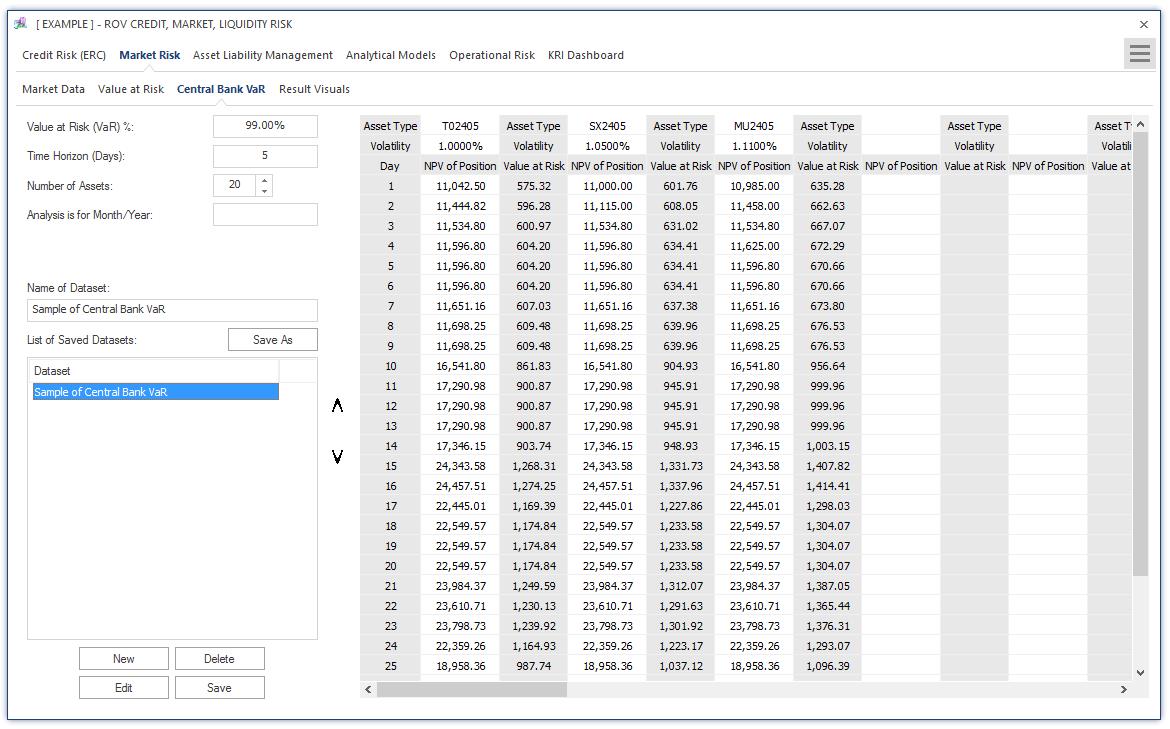
Figure 6 illustrates the PEAT utility’s ALM‐CMOL module for Asset Liability Management—Interest Rate Risk’s Input Assumptions and general Settings tab. This segment represents the analysis of ALM, or Asset Liability Management, computations. Asset Liability Management (ALM) is the practice of managing risks that arise due to mismatches between the assets and liabilities. The ALM process is a mix between risk management and strategic planning for a bank or financial institution. It is about offering solutions to mitigate or hedge the risks arising from the interaction of assets and liabilities as well as the success in the process of maximizing assets to meet complex liabilities such that it will help increase profitability.The current tab starts by obtaining, as general inputs, the bank’s regulatory capital obtained earlier from the credit risk models. In addition, the number of trading days in the calendar year of the analysis (e.g.,typically between 250 and 253 days), the local currency’s name (e.g., U.S. Dollar or Argentinian Peso), the current period when the analysis is performed and results reported to the regulatory agencies (e.g.,January 2015), the number of Value at Risk percentiles to run (e.g., 99.00%), number of scenarios to run and their respective basis point sensitivities (e.g., 100, 200, and 300 basis points, where every 100 basis points represent 1%), and number of foreign currencies in the bank’s investment portfolio. As usual, the inputs, settings, and results can be saved for future retrieval.Figure6 further illustrates the PEAT utility’s ALM‐CMOL module for Asset Liability Management. The tab is specifically for Interest Rate Sensitive Assets and Liabilities data where historical impacts of interest‐rate sensitive assets and liabilities, as well as foreign currency denominated assets and liabilities are entered, copy and pasted, or uploaded from a
database.Historical Interest Rate data is uploaded where the rows of periodic historical interest rates of
local and foreign currencies can be entered, copy and pasted, or uploaded from a database.

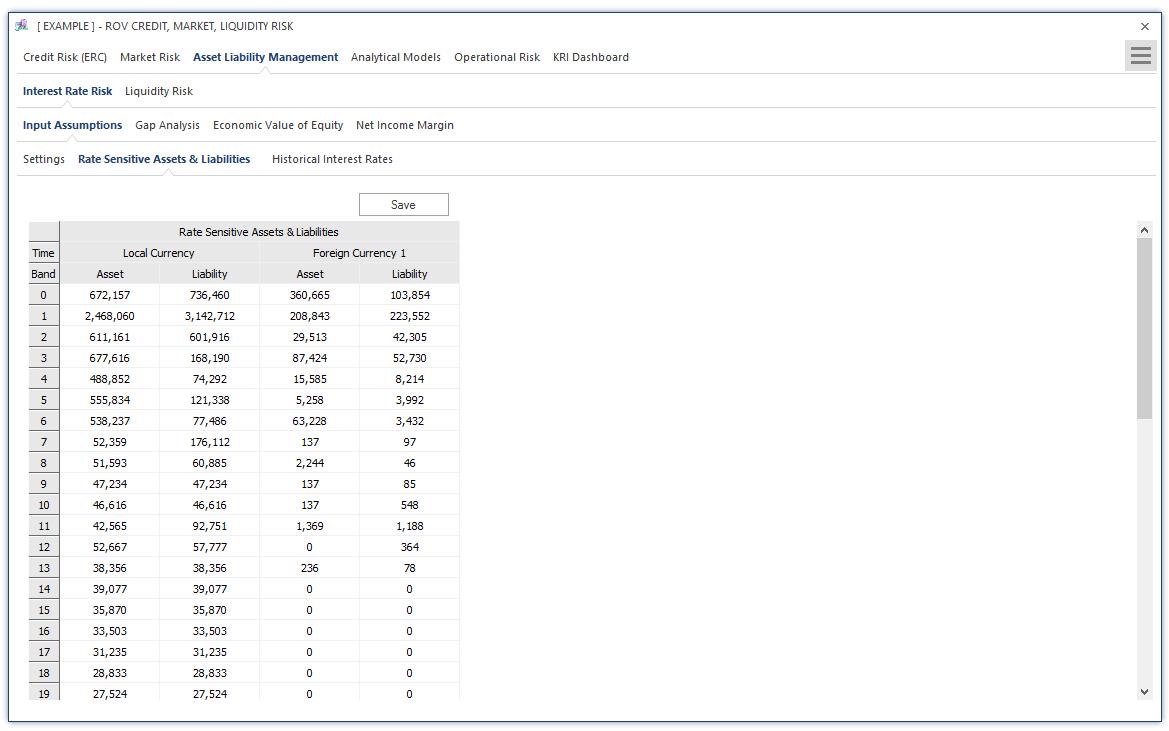
Figure 7 illustrates the Gap Analysis results of Interest Rate Risk. The results are shown in different
grids for each local currency and foreign currency. Gap Analysis is, of course, one of the most common ways of measuring liquidity position and represents the foundation for scenario analysis and stresstesting,which will be executed in subsequent tabs. The Gap Analysis results are from user inputs in the input assumptions tab. The results are presented for the user again for validation and in a more userfriendly tabular format. The Economic Value of Equity results based on interest‐rate risk computations in previous tabs. The impact on regulatory capital as denoted by VaR levels on local and foreign currencies are computed, as are the duration gaps and basis point scenarios affecting the cash flows of local and foreign currencies.

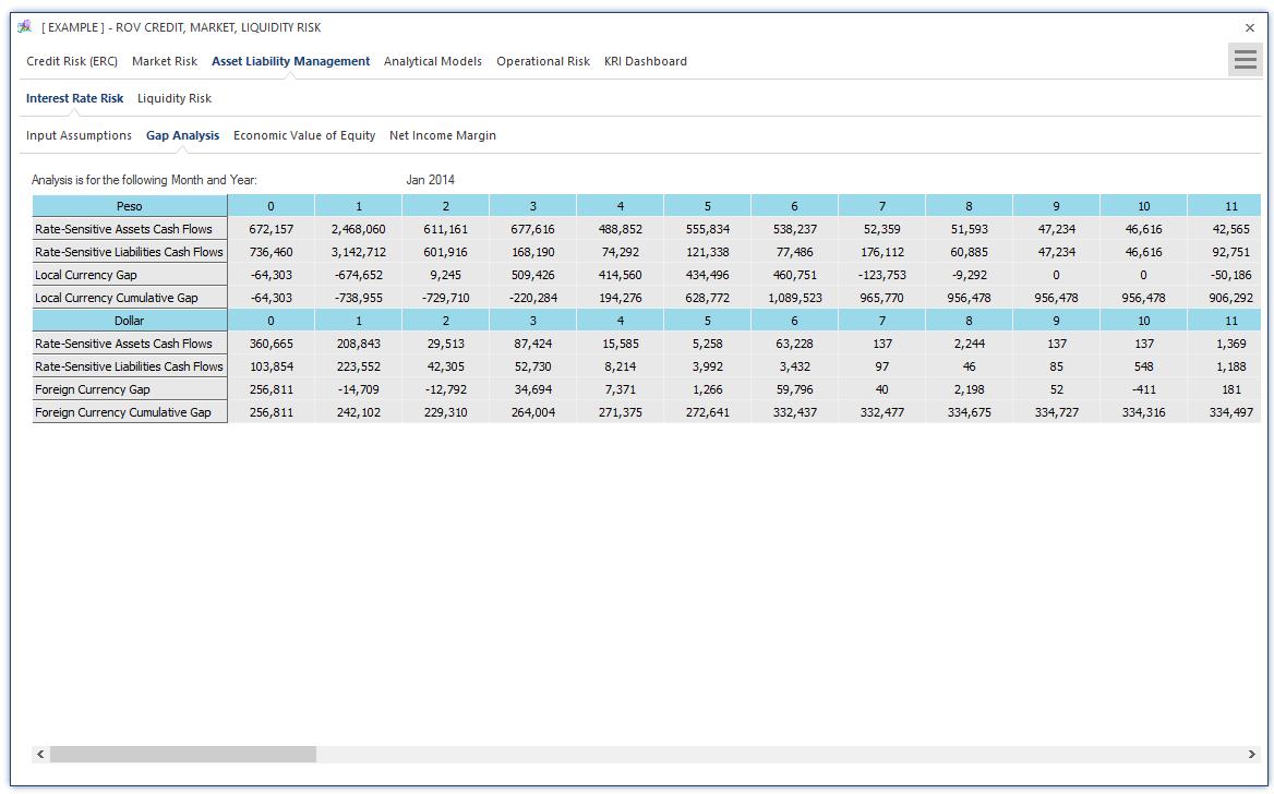
Figure 8 illustrates the Net Income Margin (NIM) Input Assumptions requirements based on interestrate risk analysis. The highlighted cells in the data grid represent user input requirements for computing the NIM model. The Economic Value of Equity and Gap Analysis calculations described above are for longer‐term interest‐rate risk analysis, whereas the NIM approach is for shorter‐term (typically 12 months) analysis of liquidity and interest‐rate risk effects on assets and liabilities.

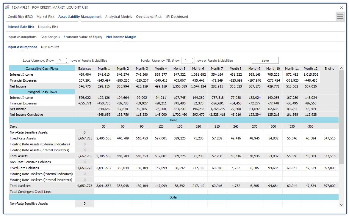
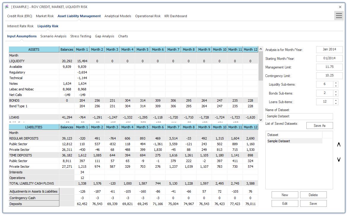
Figure 9 illustrates the PEAT utility’s ALM‐CMOL module for Asset Liability Management—Liquidity Risk Input Assumptions tab on the historical monthly balances of interest‐rate sensitive assets and liabilities. The typical time horizon is monthly for one year (12 months) where the various assets such as liquid assets (e.g., cash), bonds, and loans are listed, as well as other asset receivables. On the liabilities side, regular short‐term deposits and timed deposits are listed, separated by private versus public sectors,as well as other payable liabilities (e.g., interest payments and operations). Adjustments can also be made to account for rounding issues and accounting issues that may affect the asset and liability levels (e.g.,contingency cash levels, overnight deposits, etc.). The data grid can be set up with some basic inputs as well as the number of subsegments or rows for each category. As usual, the inputs, settings, and results can be saved for future retrieval.

The Liquidity Risk’s Scenario Analysis and Stress Testing settings can be set up to test interest‐rate sensitive assets and liabilities. The scenarios to test can be entered as data or percentage changes.Multiple scenarios can be saved for future retrieval and analysis in subsequent tabs as each saved model constitutes a stand‐alone scenario to test. Scenario analysis typically tests both fluctuations in assets and liabilities and their impacts on the portfolio’s ALM balance, whereas stress testing typically tests the fluctuations on liabilities (e.g., runs on banks, economic downturns where deposits are stressed to the lower limit) where the stressed limits can be entered as values or percentage change from the base case. Multiple stress tests can be saved for future retrieval and analysis in subsequent tabs as each saved model constitutes a stand‐alone stress test.

Figure 10 illustrates the Liquidity Risk’s Gap Analysis results. The data grid shows the results based on all the previously saved scenarios and stress test conditions. The Gap is, of course, calculated as the difference between Monthly Assets and Liabilities, accounting for any Contingency Credit Lines. The gaps for the multitude of Scenarios and Stress Tests are reruns of the same calculation based on various user inputs on values or percentage changes as described previously in the Scenario Analysis and Stress Testing sections.

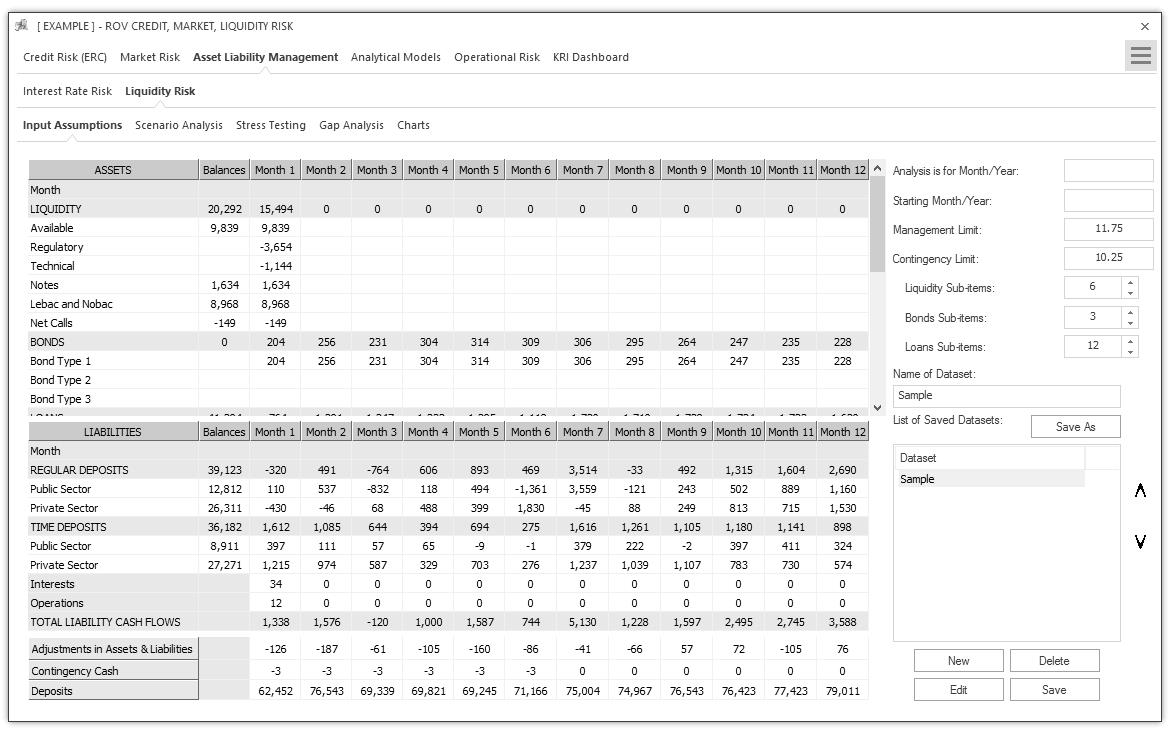
Figure 11 illustrates the Analytical Models tab with input assumptions and results. This analytical models segment is divided into Structural, Time‐Series, Portfolio, and Analytics models. The current figure shows the Structural models tab where the computed models pertain to credit risk–related model analysis categories such as Probability of Default (PD), Exposure at Default (EAD), Loss Given Default (LGD), and Volatility calculations. Under each category, specific models can be selected to run. Selected models are briefly described and users can select the number of model repetitions to run and the decimal precision levels of the results.The data grid in the Computations tab shows the area in which users would enter the relevant inputs into the selected model and the results would be Computed. As usual, selected models,inputs, and settings can be saved for future retrieval and analysis.

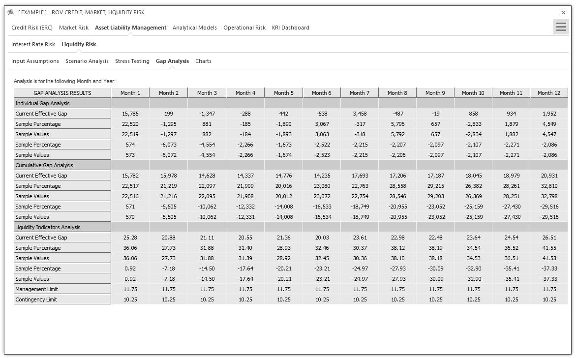
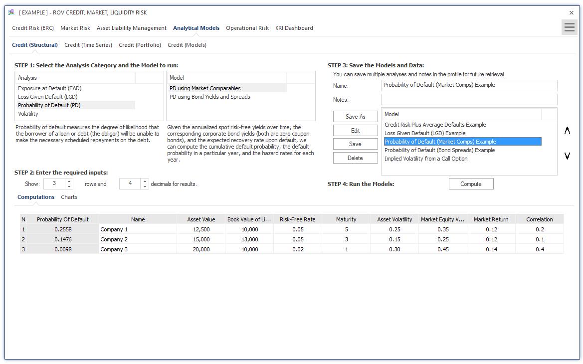
Figure 12 illustrates the Structural Analytical Models tab with visual chart results. The results computed are displayed as various visual charts such as bar charts, control charts, Pareto charts, and timeseries charts. Figure 13 illustrates the Time‐Series Analytical Models tab with input assumptions and results.The analysis category and model type is first chosen where a short description explains what the selected model does, and users can then select the number of models to replicate as well as decimal precision settings. Input data and assumptions are entered in the data grid provided (additional inputs can also be entered if required), and the results are Computed and shown. As usual, selected models,inputs, and settings can be saved for future retrieval and analysis. Figure 14 illustrates the Portfolio Analytical Models tab with input assumptions and results.The analysis category and model type is first chosen where a short description explains what the selected model does, and users can then select the number of models to replicate as well as decimal precision settings. Input data and assumptions are entered in the data grid provided (additional inputs such as a correlation matrix can also be entered if required), and the results are Computed and shown. As usual, selected models, inputs, and settings can be saved for future retrieval and analysis. Additional models are available in the Credit Models tab with input
assumptions and results. The analysis category and model type are first chosen and input data and assumptions are entered in the required inputs area (if required, users can Load Example inputs and use these as a basis for building their models), and the results are Computed and shown. Scenario tables and charts can be created by entering the From, To, and Step Size parameters, where the computed scenarios will be returned as a data grid and visual chart. As usual, selected models, inputs, and settings can be saved for future retrieval and analysis.

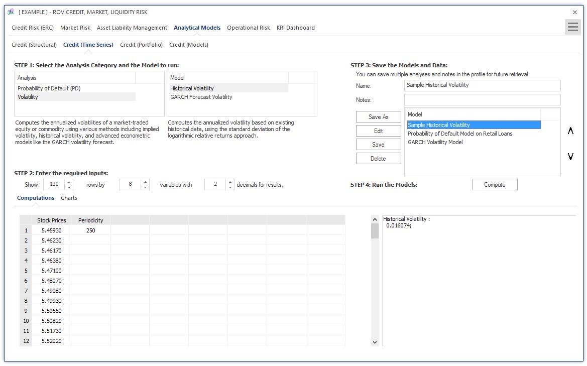
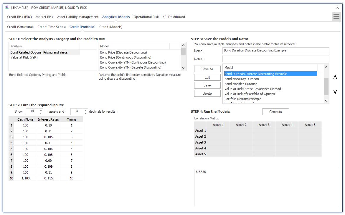
Figure 15 illustrates the Operational Risk Loss Distribution subtab. Users start at the Loss Data tab where historical loss data can be entered or pasted into the data grid. Variables include losses in the past pertaining to operational risks,segmentation by divisions and departments, business lines, dates of losses, risk categories,and so on.Users then activate the controls to select how the loss data variables are to be segmented (e.g., by risk categories and risk types and business lines), the number of simulation trials to run, and seed values to apply in the simulation if required, all by selecting the relevant variable columns.The distributional fitting routines can also be selected as required. Then the analysis can be run and distributions fitted to the data. As usual, the model settings and data can be saved for future retrieval.

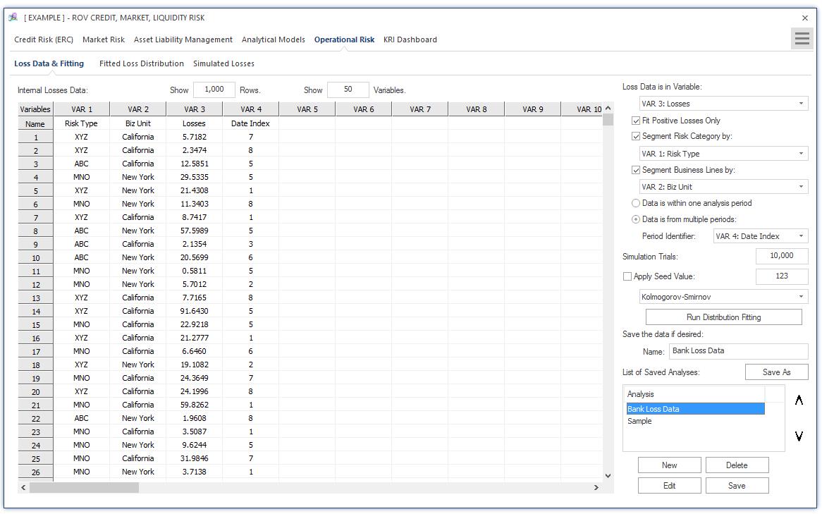
Figure 16 illustrates the Operational Risk—Fitted Loss Distribution subtab. Users start by selecting the fitting segments for setting the various risk category and business line segments, and, based on the selected segment, the fitted distributions and their p‐values are listed and ranked according to the highest p‐value to the lowest p‐value, indicating the best to the worst statistical fit to the various probability distributions. The empirical data and fitted theoretical distributions are shown graphically, and the statistical moments are shown for the actual data versus the theoretically fitted distribution’s moments.After deciding on which distributions to use, users can then run the simulations.

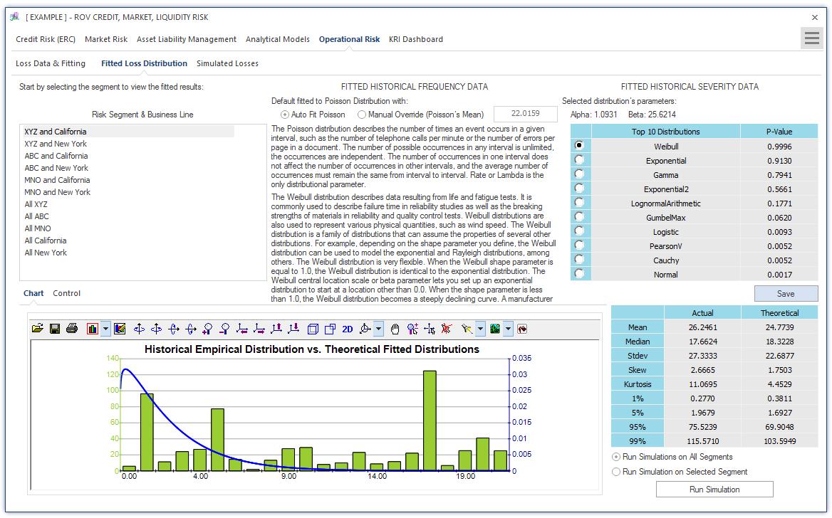
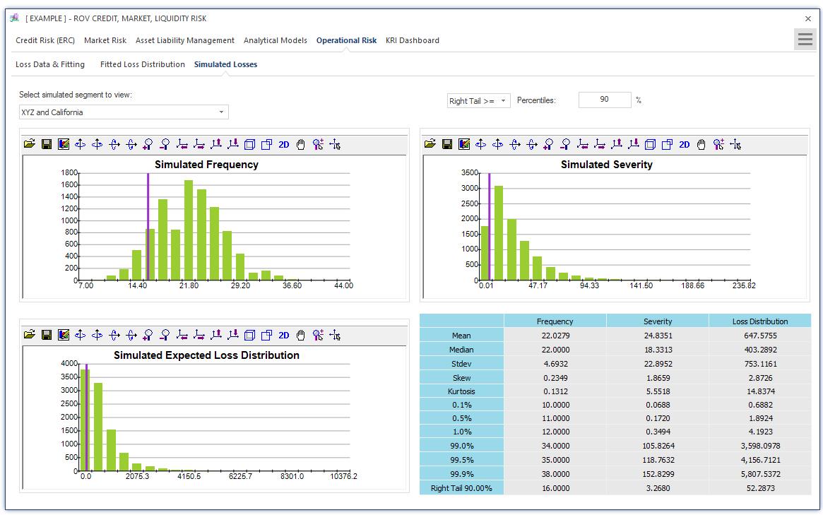
Figure 17 illustrates the Operational Risk—Simulated Losses subtab where, depending on which risk segment and business line was selected, the relevant probability distribution results from the Monte Carlo risk simulations are displayed, including the simulated results on Frequency, Severity, and the multiplication between frequency and severity, termed Expected Loss Distribution, as well as the Extreme Value Distribution of Losses (this is where the extreme losses in the data set are fitted to the extreme value distributions—see the case study for details on extreme value distributions and their mathematical models). Each of the distributional charts has its own confidence and percentile inputs where users can select one‐tail (right‐tail or left‐tail) or two‐tail confidence intervals and enter the percentiles to obtain the confidence values (e.g., user can enter right‐tail 99.90% percentile to receive the Value at Risk confidence value of the worst‐case losses on the left tail’s 0.10%).