Correlations and Correlated Simulation with Copulas

• By Admin
• October 1, 2014
• Comments Off on Correlations and Correlated Simulation with Copulas

The Basics of Correlations
The correlation coefficient is a measure of the strength and direction of the relationship between two variables, and it can take on any value between –1.0 and +1.0. That is, the correlation coefficient can be decomposed into its sign (positive or negative relationship between two variables) and the magnitude or strength of the relationship (the higher the absolute value of the correlation coefficient, the stronger the relationship). The correlation coefficient can be computed in several ways. The first approach is to manually compute the correlation, r, of two variables, x and y, using:

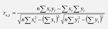
The second approach is to use Excel’s CORREL function. For instance, if the 10 data points for x and y are listed in cells A1:B10, then the Excel function to use is CORREL (A1:A10, B1:B10).

The third approach is to run Risk Simulator │ Analytical Tools │ Distributional Fitting (Multi- Variable), and the resulting correlation matrix will be computed.

It is important to note that correlation does not imply causation. Two completely unrelated random variables might display some correlation but this does not imply any causation between the two (e.g., sunspot activity and events in the stock market are whitenoise correlated but there is no causation between the two).

There are two general types of correlations: parametric and nonparametric correlations. Pearson’s correlation coefficient is the most common correlation measure and is usually referred to simply as the correlation coefficient. However, Pearson’s correlation is a parametric measure, which means that it requires both correlated variables to have an underlying normal distribution and that the relationship between the variables is linear. When these conditions are violated, which is often the case in Monte Carlo simulation, the nonparametric counterparts become more important. Spearman’s rank correlation and Kendall’s tau are the two alternatives to the Pearson’s correlation. The Spearman correlation is most commonly used and is most appropriate when applied in the context of Monte Carlo simulation––there is no dependence on normal distributions or linearity, meaning that correlations between different variables with different distribution can be applied. To compute the Spearman correlation, first rank all the x and y variable values and then apply the Pearson’s correlation computation.

Correlations affect risk, as can be seen in a portfolio where risk is diversified. A portfolio’s risk is typically computed as:

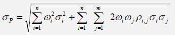
where ρi,j are the respective cross-correlations between the asset classes, σi,j are the individual asset classes’ risk levels, and ωi,j are the respective weights or capital allocation across each project or asset class. Hence, if the cross-correlations are negative, there are risk diversification effects, and the portfolio risk decreases. In contrast, when the correlations are positive, the portfolio’s risk increases. See the next section on the effects of correlations in Monte Carlo risk simulation, and specifically, see Figures 1 and 2 for more details.

The Effects of Correlations in Monte Carlo Risk Simulation
Although the computations required to correlate variables in a stochastic simulation are complex, the resulting effects are fairly clear. Figure 1 shows a simple correlation model (Correlation Effects Model in the Risk Simulator examples folder). The calculation for revenue is simply price multiplied by quantity. The same model is replicated for no correlations, positive correlation (+0.8), and negative correlation (–0.8) between price and quantity.

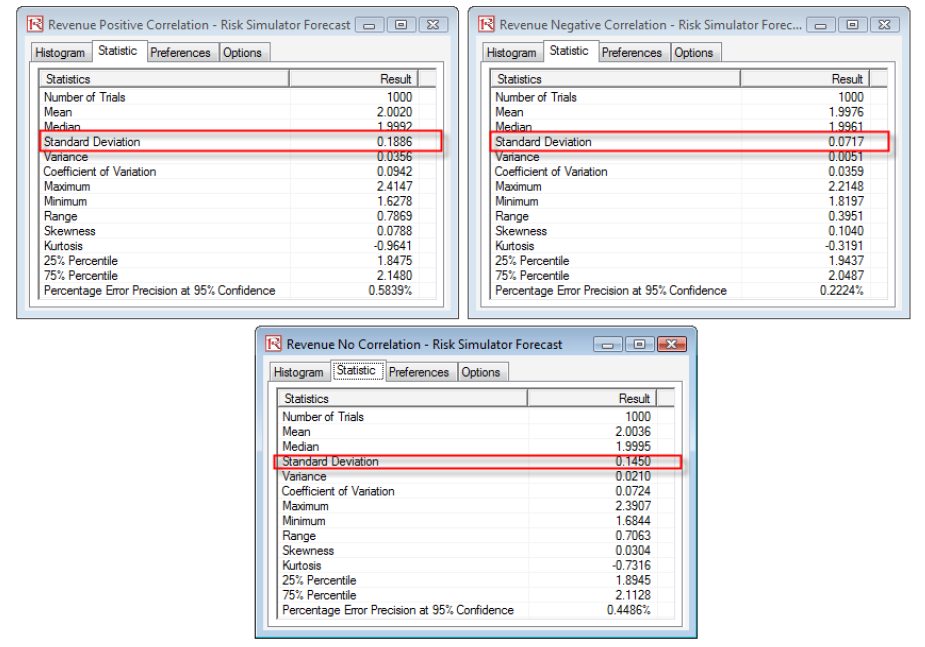
The resulting statistics are shown in Figure 2. Notice that the standard deviation of the model without correlations is 0.1450, compared to 0.1886 for the positive correlation model and 0.0717 for the negative correlation model. That is, for simple models, negative correlations tend to reduce the average spread of the distribution and create a tight and more concentrated forecast distribution as compared to positive correlations with larger average spreads. However, the mean remains relatively stable. This fact implies that correlations do little to change the expected value of projects but can reduce or increase a project’s risk.

Figure 1. Illustrates a simple model of price multiplied by quantity to obtain the revenue amount. The same model is replicated three times, and each model bears different correlations between price and quantity (no correlation, positive +0.8 correlation, and negative –0.8 correlation), such that we can test the effect on the revenue output forecast.

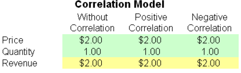
Figure 2. Illustrates the resulting output forecasts of the three revenues shown in Figure 1. The first moment remains relatively unchanged, while correlations have unknown effects on the third and fourth moments (these moments depend on the input assumptions’ skew and kurtosis depending on distributional type). However, we do know that correlations tend to affect the second moment (risk or spread/width of the distribution). In a positively related model (e.g., price multiplied by quantity), negative correlations will reduce risk while positive correlations will increase risk. The opposite is true in a negatively related model (e.g., revenue minus cost equals income) where positive correlations will reduce risk while negative correlations will increase risk.

Applying Correlations in Risk Simulator
Correlations can be applied in Risk Simulator in several ways:

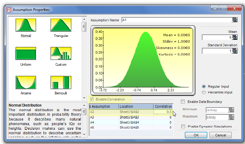
• When defining assumptions (Risk Simulator │ Set Input Assumption), simply enter the correlations into the correlation matrix grid in the Distribution Gallery (Figure 3).
• With existing data, run the Multi-Fit tool, Risk Simulator │ Analytical Tools │ Distributional Fitting (Multi-Variable), to perform distributional fitting and to obtain the correlation matrix between pairwise variables. If a simulation profile exists, the assumptions fitted will automatically contain the relevant correlation values.
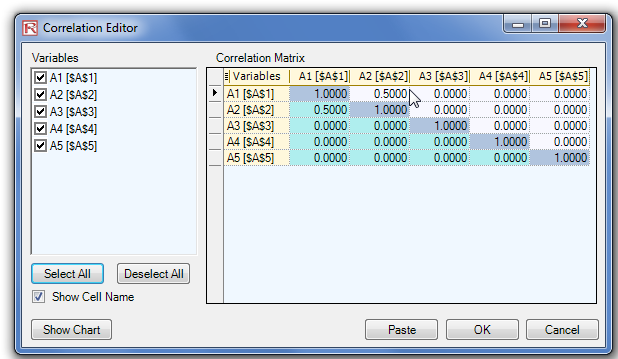
• With existing assumptions, you can click on Risk Simulator │Analytical Tools │Edit Correlations to enter the pairwise correlations of all the assumptions directly in one user interface (Figure 3).

Note that the correlation matrix must be positive definite. That is, the correlation must be mathematically valid. For instance, suppose you are trying to correlate three variables: grades of graduate students in a particular year, the number of beers they consume a week, and the number of hours they study a week. One would assume that the following correlation relationships exist:

Grades and Beer: – The more they drink, the lower the grades (no-show on exams)
Grades and Study: + The more they study, the higher the grades
Beer and Study: – The more they drink, the less they study (drunk and partying all the time)

However, if you input a negative correlation between Grades and Study, and assuming that the correlation coefficients have high magnitudes, the correlation matrix will be nonpositive definite. It would defy logic, correlation requirements, and matrix mathematics. However, smaller coefficients can sometimes still work even with the bad logic. When a nonpositive definite or bad correlation matrix is entered, Risk Simulator will automatically inform you, and offers to adjust these correlations to something that is semipositive definite while still maintaining the overall structure of the co rrelation relationship (the same signs as well as the same relative strengths).

Figure 3. You can set correlations in the Input Assumption dialog or in the Edit Correlation tool in Risk Simulator.

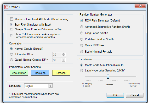
Random Number Generation, Monte Carlo versus Latin Hypercube, and Correlation Copulas Starting with version 2011/2012, there are 6 Random Number Generators, 3 Correlation Copulas, and 2 Simulation Sampling Methods to choose from (Figure 4). These preferences are set through Risk Simulator | Options. The Random Number Generator (RNG) is at the heart of any simulation software. Based on the random number generated, different mathematical distributions can be constructed. The default method is the ROV Risk Simulator proprietary methodology, which provides the best and most robust random numbers. As noted, there are 6 supported random number generators and, in general, the ROV Risk Simulator default method and the Advanced Subtractive Random Shuffle method are the two approaches recommended for use. Do not apply the other methods unless your model or analytics specifically calls for their use, and even then, we advise testing the results against these two recommended approaches. The further down the list of RNGs, the simpler the algorithm and the faster it runs, in comparison with the more robust results from RNGs further up the list.

In the Correlations section, three methods are supported: the Normal Copula, T-Copula, and Quasi-Normal Copula. These methods rely on mathematical integration techniques, and when in doubt, the normal copula provides the safest and most conservative results. The t-copula provides for extreme values in the tails of the simulated distributions, whereas the quasinormal copula returns results that are between the values derived by the other two methods.

In the Simulation methods section, Monte Carlo Simulation (MCS) and Latin Hypercube Sampling (LHS) methods are supported. Note that Copulas and other multivariate functions are not compatible with LHS because LHS can be applied to a single random variable but not over a joint distribution. In reality, LHS has very limited impact on the model output’s accuracy the more distributions there are in a model since LHS only applies to distributions individually. The benefit of LHS is also eroded if one does not complete the number of samples specified at the beginning, that is, if one halts the simulation run in mid-simulation. LHS also applies a heavy burden on a simulation model with a large number of inputs because it needs to generate and organize samples from each distribution prior to running the first sample from a distribution. This necessity can cause a long delay in running a large model without providing much more additional accuracy. Finally, LHS is best applied when the distributions are well behaved and symmetrical and without any correlations. Nonetheless, LHS is a powerful approach that yields a uniformly sampled distribution, where MCS can sometimes generate lumpy distributions (sampled data can sometimes be more heavily concentrated in one area of the distribution) as compared to a more uniformly sampled distribution (every part of the distribution will be sampled) when LHS is applied.

Figure 4. Risk Simulator’s Options user interface where you can set or change the correlation copulas.