Decision Tree and Related Analytics

• By Admin
• September 10, 2014
• Comments Off on Decision Tree and Related Analytics

Decision Tree
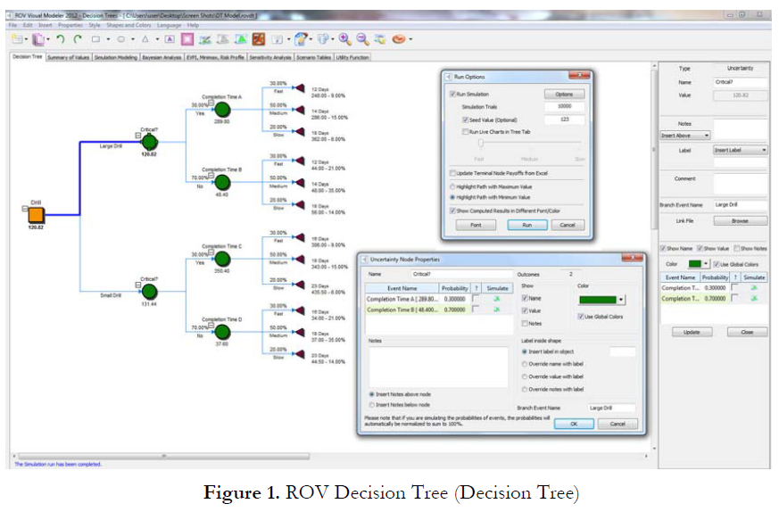
Risk Simulator | Decision Tree runs the Decision Tree module (Figure 1), which is used to create and value decision tree models. Additional advanced methodologies and analytics are also included:

• Decision Tree Models
• Monte Carlo risk simulation
• Sensitivity Analysis
• Scenario Analysis
• Bayesian (Joint and Posterior Probability Updating)
• Expected Value of Information
• MINIMAX
• MAXIMIN
• Risk Profiles

The following are some main quick getting started tips and procedures for using this
intuitive tool:

• There are 11 localized languages available in this module and the current language can be changed through the Language menu.
• Insert Option nodes or Insert Terminal nodes by first selecting any existing node and then clicking on the option node icon (square) or terminal node icon (triangle), or use the functions in the Insert menu.
• Modify individual Option Node or Terminal Node properties by double-clicking on a node. Sometimes when you click on a node, all subsequent child nodes are also selected (this allows you to move the entire tree starting from that selected node). If you wish to select only that node, you can have to click on the empty background and click back on that node to select it individually. Also, you can move individual nodes or the entire tree started from the selected node depending on the current setting (right-click, or in the Edit menu, select Move Nodes Individually or Move Nodes Together).
• The following are some brief descriptions of the things that can be customized and configured in the node properties user interface. It is simplest to try different settings for each of the following to see its effects in the Strategy Tree:
• Name: Name shown above the node.
• Value: Value shown below the node.
• Excel Link: Links the value from an Excel spreadsheet’s cell.
• Notes: Notes can be inserted above or below a node.
• Show in Model: Show any combinations of Name, Value, and Notes.
• Local Color versus Global Color: Node colors can be changed locally to a node or globally.
• Label Inside Shape: Text can be placed inside the node (you may need to make the node wider to accommodate longer text).
• Branch Event Name: Text can be placed on the branch leading to the node to indicate the event leading to this node.
• Select Real Options: A specific real option type can be assigned to the current node. Assigning real options to nodes allows the tool to generate a list of required input variables.
• Global Elements are all customizable, including elements of the Strategy Tree’s Background, Connection Lines, Option Nodes, Terminal Nodes, and Text Boxes. For instance, the following settings can be changed for each of the elements:
• Font settings on Name, Value, Notes, Label, Event names.
• Node Size (minimum and maximum height and width).
• Borders (line styles, width, and color).
• Shadow (colors and whether to apply a shadow or not).
• Global Color.
• Global Shape.
• The Edit menu’s View Data Requirements Window command opens a docked window on the right of the Strategy Tree such that when an option node or terminal node is selected, the properties of that node will be displayed and can be updated directly. This feature provides an alternative to double-clicking on a node each time.
• Example Files are available in the File menu to help you get started on building Strategy Trees.
• Protect File from the File menu allows the Strategy Tree to be encrypted with up to a 256-bit password encryption. Be careful when a file is being encrypted because if the password is lost, the file can no longer be opened.
• Capturing the Screen or printing the existing model can be done through the File menu. The captured screen can then be pasted into other software applications.
• Add, Duplicate, Rename, and Delete a Strategy Tree can be performed through right-clicking the Strategy Tree tab or the Edit menu.
• You can also Insert File Link and Insert Comment on any option or terminal node, or Insert Text or Insert Picture anywhere in the background or canvas area.
• You can Change Existing Styles or Manage and Create Custom Styles of your Strategy Tree (this includes size, shape, color schemes, and font size/color specifications of the entire Strategy Tree).
• Insert Decision, Insert Uncertainty, or Insert Terminal nodes by selecting any existing node and then clicking on the decision node icon (square), uncertainty node icon (circle), or terminal node icon (triangle), or use the functionalities in the Insert menu.
• Modify individual Decision, Uncertainty, or Terminal nodes’ properties by double-clicking on a node. The following are some additional unique items in the Decision Tree module that can be customized and configured in the node properties user interface:
• Decision Nodes: Custom Override or Auto Compute the value on a node. The automatically compute option is set as
  default and when you click Run on a completed Decision Tree model, the decision nodes will be updated with the results.
• Uncertainty Nodes: Event Names, Probabilities, and Set Simulation Assumptions. You can add probability event names, probabilities, and simulation assumptions only after the uncertainty branches are created.
• Terminal Nodes: Manual Input, Excel Link, and Set Simulation Assumptions. The terminal event payoffs can be entered manually or linked to an Excel cell (e.g., if you have a large Excel model that computes the payoff, you can link the model to this Excel model’s output cell) or set probability distributional assumptions for running simulations.
• View Node Properties Window is available from the Edit menu and the selected node’s properties will update when a node is selected.
• The Decision Tree module also comes with the following advanced analytics:
• Monte Carlo Simulation Modeling on Decision Trees
• Bayes Analysis for obtaining posterior probabilities
• Expected Value of Perfect Information, MINIMAX and MAXIMIN Analysis, Risk Profiles, and Value of Imperfect Information
• Sensitivity Analysis
• Scenario Analysis
• Utility Function Analysis

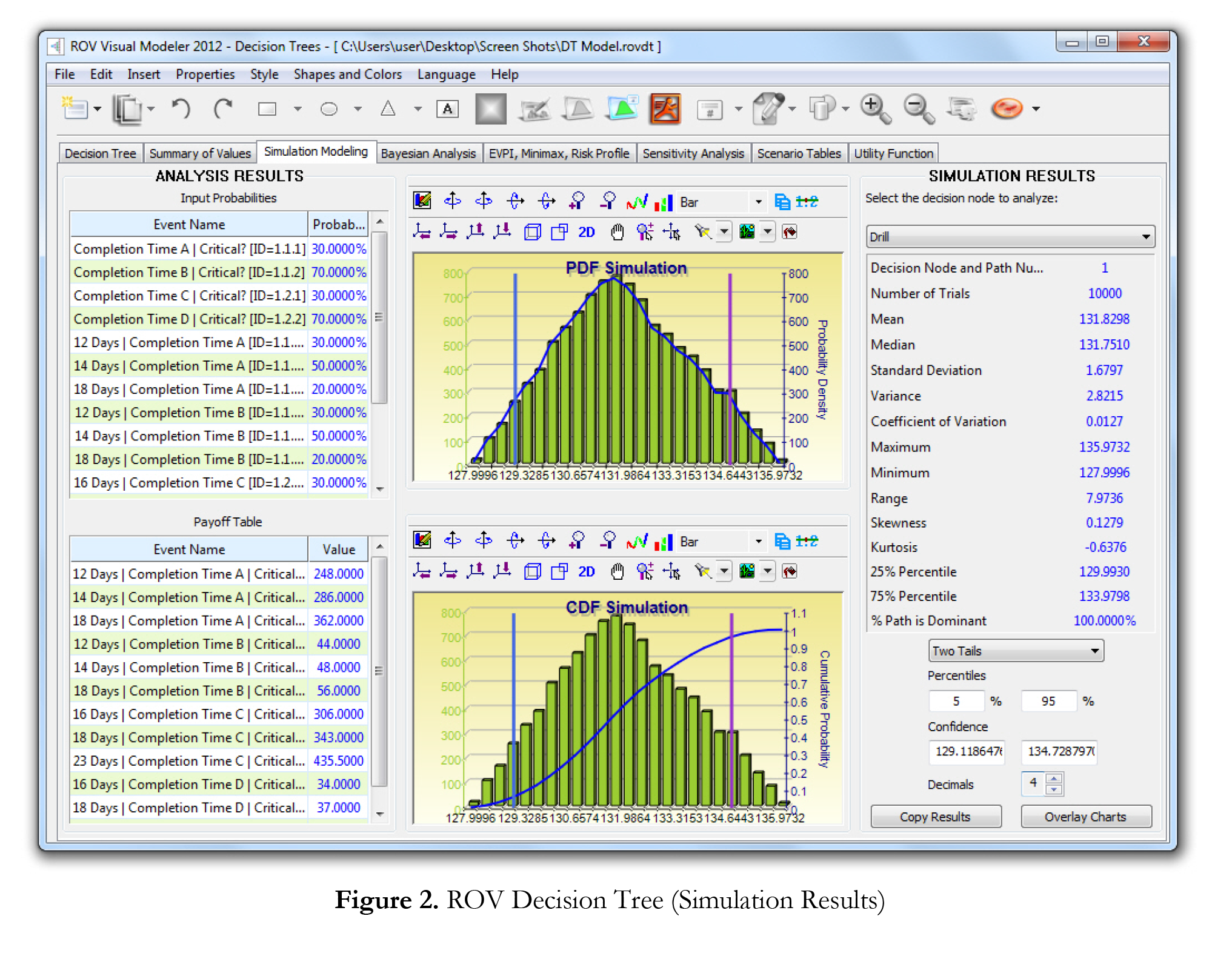
Simulation Modeling
This tool runs Monte Carlo risk simulation on the decision tree (Figure 2). It allows you to set probability distributions as input assumptions for running simulations. You can either set an assumption for the selected node or set a new assumption and use this new assumption (or use previously created assumptions) in a numerical equation or formula. For example, you can set a new assumption called Normal (e.g., normal distribution with a mean of 100 and standard deviation of 10) and run a simulation in the decision tree, or use this assumption in an equation such as (100*Normal+15.25). Create your own model in the numerical expression box. You can use basic computations or add existing variables into your equation by double-clicking on the list of existing variables. New variables can be added to the list as required either as numerical expressions or assumptions.

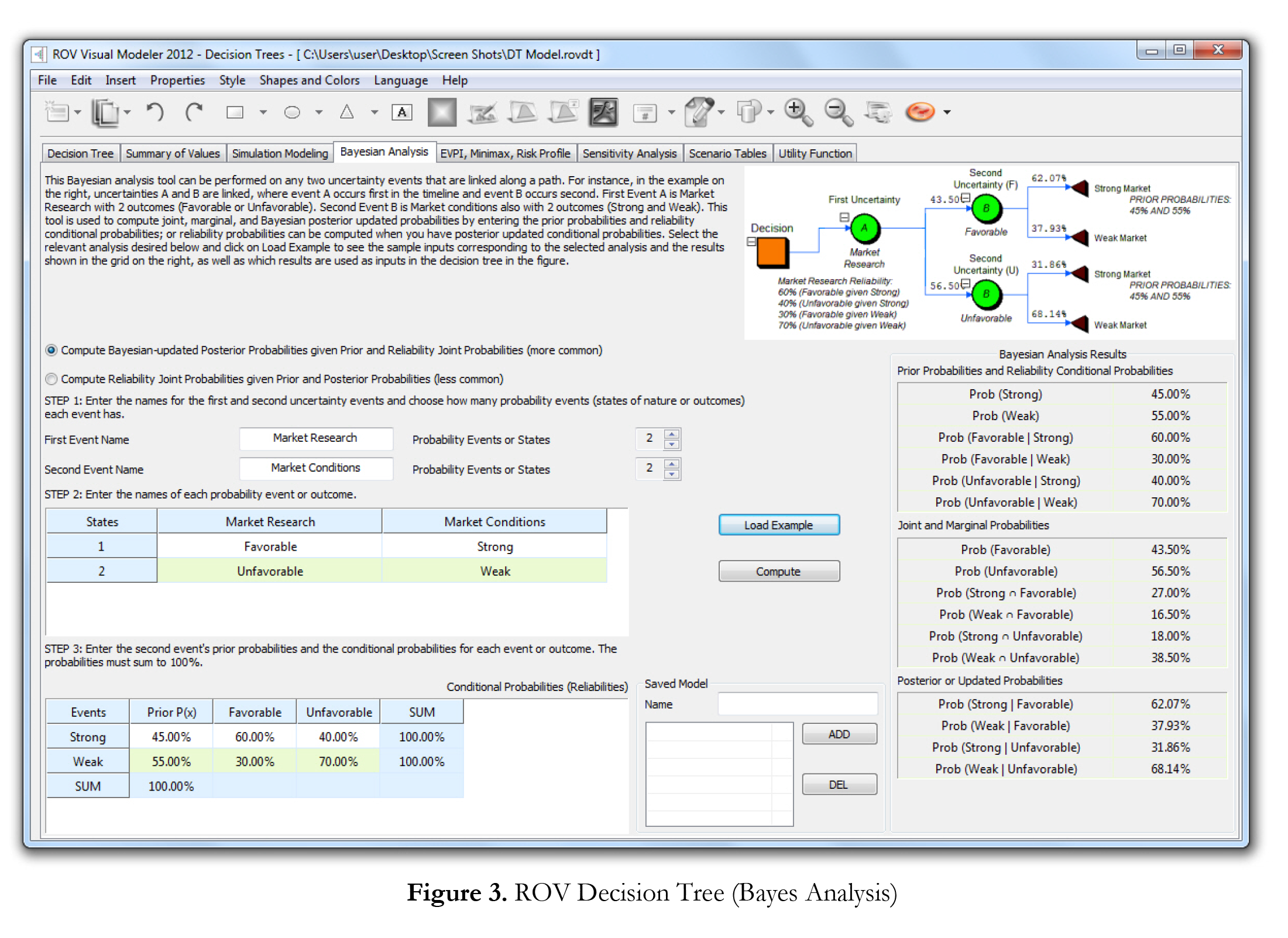
Bayes Analysis
The Bayesian analysis tool (Figure 3) can be used on any two uncertainty events that are linked along a path. For instance, in the example on the right in Figure 3, uncertainties A and B are linked, where event A occurs first in the timeline and event B occurs second. First Event A is Market Research with 2 outcomes (Favorable or Unfavorable). Second Event B is Market Conditions also with 2 outcomes (Strong and Weak). This tool is used to compute joint, marginal, and Bayesian posterior updated probabilities by entering the prior probabilities and reliability conditional probabilities; or reliability probabilities can be computed when you have posterior updated conditional probabilities. Select the relevant analysis desired and click on Load Example to see the sample inputs corresponding to the selected analysis and the results shown in the grid on the right, as well as which results are used as inputs in the decision tree in the figure.

Quick Procedures

• STEP 1: Enter the names for the first and second uncertainty events and choose how many probability events (states of nature or outcomes) each event has.
• STEP 2: Enter the names of each probability event or outcome.
• STEP 3: Enter the second event’s prior probabilities and the conditional probabilities for each event or outcome. The probabilities must sum to 100%.

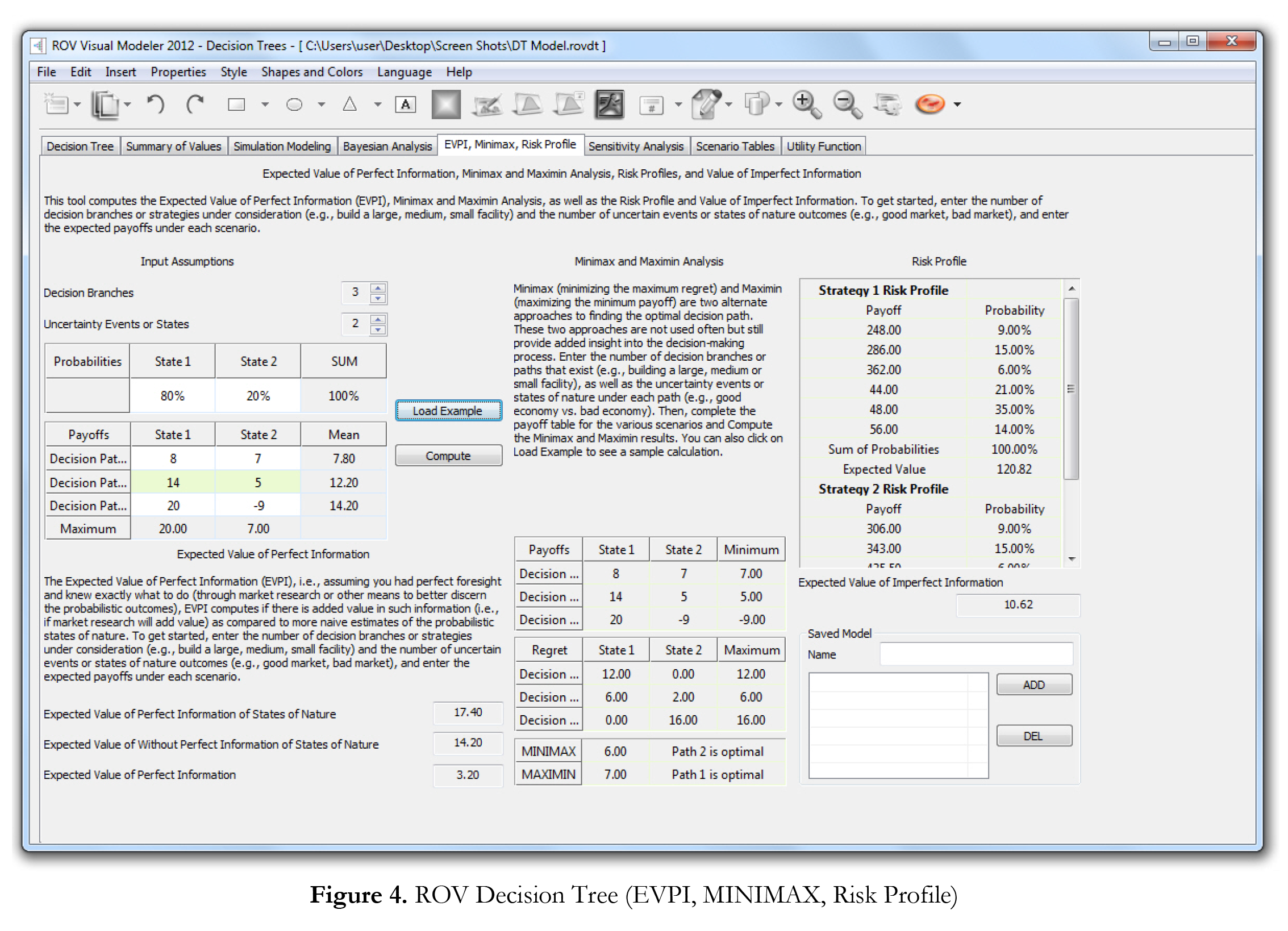
Expected Value of Perfect Information, MINIMAX and MAXIMIN Analysis, Risk Profiles, and Value of Imperfect Information
This tool (Figure 4) computes the Expected Value of Perfect Information (EVPI), MINIMAX and MAXIMIN Analysis, as well as the Risk Profile and the Value of Imperfect Information. To get started, enter the number of decision branches or strategies under consideration (e.g., build a large, medium, or small facility), the number of uncertain events or states of nature outcomes (e.g., good market, bad market), and the expected payoffs under each scenario.

The Expected Value of Perfect Information (EVPI), assuming you had perfect foresight and knew exactly what to do (through market research or other means to better discern the probabilistic outcomes), computes if there is added value in such information (i.e., if market research will add value) as compared to more naive estimates of the probabilistic states of nature. To get started, enter the number of decision branches or strategies under consideration (e.g., build a large, medium, or small facility) and the number of uncertain events or states of nature outcomes (e.g., good market, bad market), and enter the expected payoffs under each scenario.

MINIMAX (minimizing the maximum regret) and MAXIMIN (maximizing the minimum payoff) are two alternate approaches to finding the optimal decision path. These two approaches are not used often but still provide added insight into the decision-making process. Enter the number of decision branches or paths that exist (e.g., building a large, medium, or small facility), as well as the uncertainty events or states of nature under each path (e.g., good economy vs. bad economy). Then, complete the payoff table for the various scenarios and Compute the MINIMAX and MAXIMIN results. You can also click on Load Example to see a sample calculation.

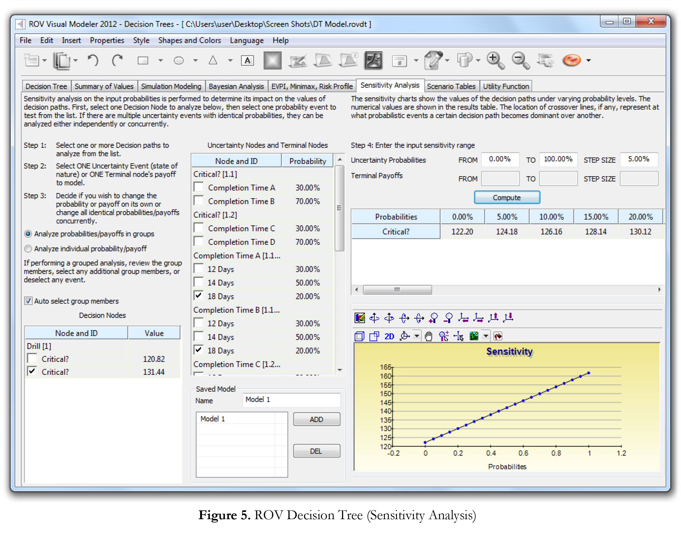
Sensitivity
Sensitivity analysis (Figure 5) on the input probabilities is performed to determine the impact of inputs on the values of decision paths. First, select one Decision Node to analyze, and then select one probability event to test from the list. If there are multiple uncertainty events with identical probabilities, they can be analyzed either independently or concurrently. The sensitivity charts show the values of the decision paths under varying probability levels. The numerical values are shown in the results table. The location of crossover lines, if any, represents at what probabilistic events a certain decision path becomes dominant over another.

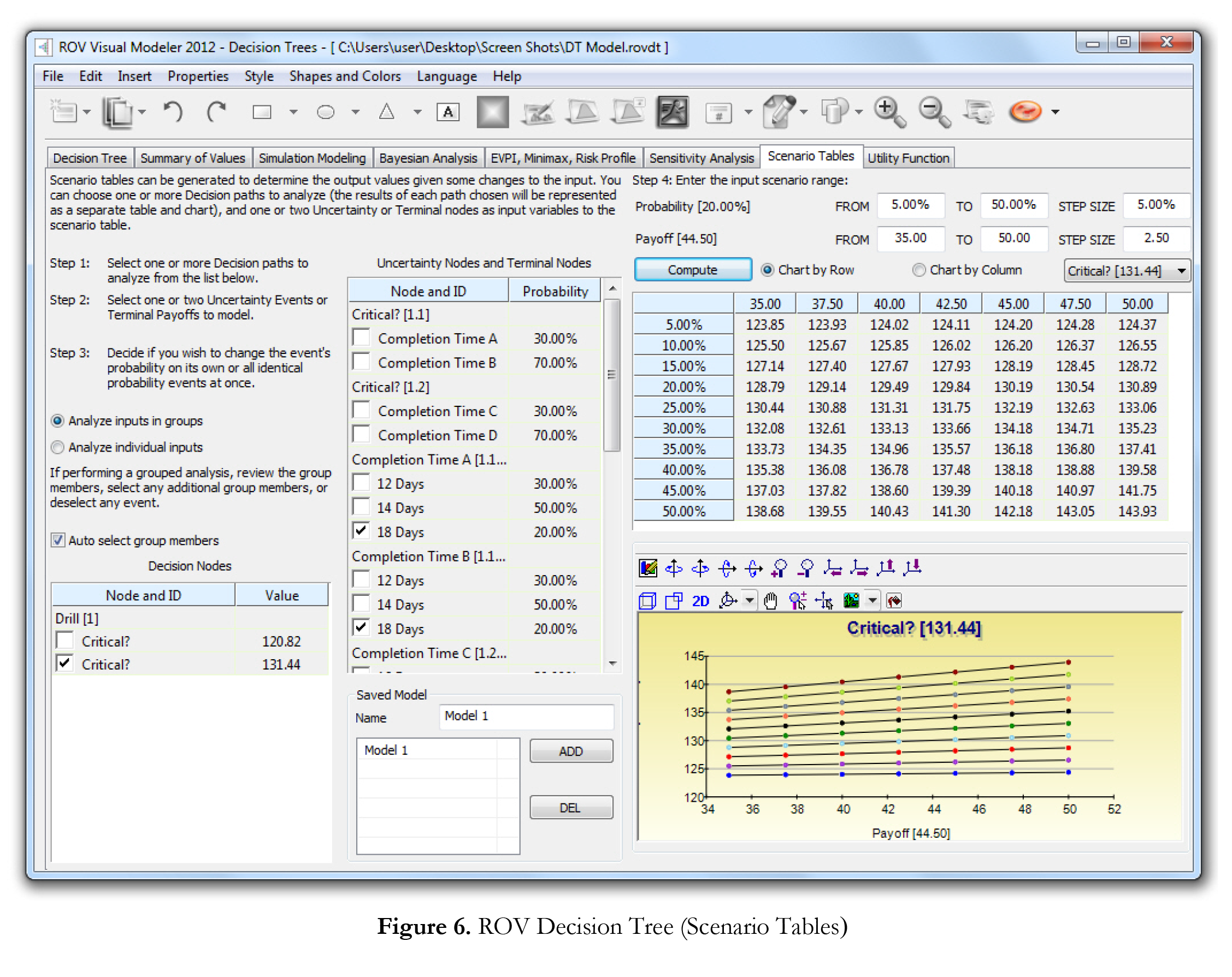
Scenario Tables
Scenario tables (Figure 6) can be generated to determine the output values given some changes to the input. You can choose one or more Decision paths to analyze (the results of each path chosen will be represented as a separate table and chart) and one or two Uncertainty or Terminal nodes as input variables to the scenario table.

Quick Procedures

• Select one or more Decision paths to analyze from the list below.
• Select one or two Uncertainty Events or Terminal Payoffs to model.
• Decide if you wish to change the event’s probability on its own or all identical probability events at once.
• Enter the input scenario range.

Utility Function Generation
Utility functions (Figure 7), or U(x), are sometimes used in place of expected values of terminal payoffs in a decision tree. They can be developed two ways: using tedious and detailed experimentation of every possible outcome or an exponential extrapolation method (used here). They can be modeled for a decision maker who is risk-averse (downsides are more disastrous or painful than an equal upside potential), risk-neutral (upsides and downsides have equal attractiveness), or riskloving (upside potential is more attractive). Enter the minimum and maximum expected value of your terminal payoffs and the number of data points in between to compute the utility curve and table.

If you had a 50:50 gamble where you either earn $X or lose -$X/2 versus not playing and getting a $0 payoff, what would this $X be? For example, if you are indifferent between a bet where you can win $100 or lose -$50 with equal probability compared to not playing at all, then your X is $100. Enter the X in the Positive Earnings box. Note that the larger X is, the less risk-averse you are, whereas a smaller X indicates that you are more risk-averse.

Enter the required inputs, select the U(x) type, and click Compute Utility to obtain the results. You can also apply the computed U(x) values to the decision tree to rerun it, or revert the tree back to using expected values of the payoffs.