Detecting and Fixing Some Common Forecasting Problems: Heteroskedasticity, Multicollinearity, and Autocorrelation

• By Admin
• September 24, 2014
• Comments Off on Detecting and Fixing Some Common Forecasting Problems: Heteroskedasticity, Multicollinearity, and Autocorrelation

Detecting and Fixing Heteroskedasticity

Several tests exist to check for the presence of heteroskedasticity. These tests also are applicable for testing misspecifications and nonlinearities. The simplest approach is to graphically represent each independent variable against the dependent variable. Another approach is to apply one of the most widely used models, the White’s test, where the test is based on the null hypothesis of no heteroskedasticity against an alternate hypothesis of heteroskedasticity of some unknown general form. The test statistic is computed by an auxiliary or secondary regression, where the squared residuals or errors from the first regression are regressed on all possible (and nonredundant) cross products of the regressors.
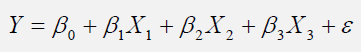
For example, suppose the following regression is estimated:

Error! Objects cannot be created from editing field codes.

The test statistic is then based on the auxiliary regression of the errors (Є):

Error! Objects cannot be created from editing field codes.

The nR2 statistic is the White’s test statistic, computed as the number of observations (n) times the centered R-squared from the test regression. White’s test statistic is asymptotically distributed as a x2 with degrees of freedom equal to the number of independent variables (excluding the constant) in the test regression.

The White’s test is also a general test for model misspecification, because the null hypothesis underlying the test assumes that the errors are both homoskedastic and independent of the regressors and that the linear specification of the model is correct. Failure of any one of these conditions could lead to a significant test statistic. Conversely, a nonsignificant test statistic implies that none of the three conditions is violated. For instance, the resulting F-statistic is an omitted variable test for the joint significance of all cross products, excluding the constant.

One method to fix heteroskedasticity is to make it homoskedastic by using a weighted least squares (WLS) approach. For instance, suppose the following is the original regression
equation:

Further suppose that X2 is heteroskedastic. Then transform the data used in the regression into:

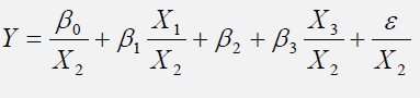
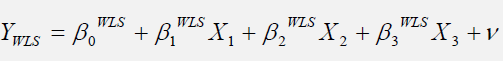
The model can be redefined as the following WLS regression:

Alternatively, the Park’s test can be applied to test for heteroskedasticity and to fix it. The Park’s test model is based on the original regression equation, uses its errors, and creates an auxiliary regression that takes the form of:

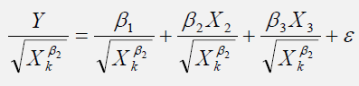
Suppose β2 is found to be statistically significant based on a t-test, then heteroskedasticity is found to be present in the variable Xk,i. The remedy, therefore, is to use the following regression specification:

Detecting and Fixing Multicollinearity
Multicollinearity exists when there is a linear relationship between the independent variables. When this occurs, the regression equation cannot be estimated at all. In near collinearity situations, the estimated regression equation will be biased and provide inaccurate results. This situation is especially true when a step-wise regression approach is used, where the statistically significant independent variables will be thrown out of the regression mix earlier than expected, resulting in a regression equation that is neither efficient nor accurate. As an example, suppose the following multiple regression analysis exists, where Error! Objects cannot be created from editing field codes.. Then the estimated slopes can be calculated through

Error! Objects cannot be created from editing field codes.

Now suppose that there is perfect multicollinearity, that is, there exists a perfect linear relationship between X2 and X3, such that Error! Objects cannot be created from editing field codes. for all positive values of λ. Substituting this linear relationship into the slope calculations for β2, the result is indeterminate. In other words, we have

Error! Objects cannot be created from editing field codes.

The same calculation and results apply to β3, which means that the multiple regression analysis breaks down and cannot be estimated given a perfect collinearity condition.

One quick test of the presence of multicollinearity in a multiple regression equation is that the R-squared value is relatively high while the t-statistics are relatively low. Another quick test is to create a correlation matrix between the independent variables. A high cross correlation indicates a potential for multicollinearity. The rule of thumb is that a correlation with an absolute value greater than 0.75 is indicative of severe multicollinearity. Another test for multicollinearity is the use of the variance inflation factor (VIF), obtained by regressing each independent variable to all the other independent variables, obtaining the R-squared value and calculating the VIF of that variable by estimating:

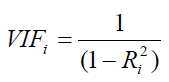
A high VIF value indicates a high R-squared near unity. As a rule of thumb, a VIF value greater than 10 is usually indicative of destructive multicollinearity.

Detecting and Fixing Autocorrelation
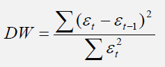
One very simple approach to test for autocorrelation is to graph the time series of a regression equation’s residuals. If these residuals exhibit some cyclicality, then autocorrelation exists. Another more robust approach to detect autocorrelation is the use of the Durbin-Watson statistic, which estimates the potential for a first-order autocorrelation. The Durbin-Watson test also identifies model misspecification, that is, if a particular time-series variable is correlated to itself one period prior. Many time-series data tend to be autocorrelated to their historical occurrences. This relationship can be due to multiple reasons, including the variables’ spatial relationships (similar time and space), prolonged economic shocks and events, psychological inertia, smoothing, seasonal adjustments of the data, and so forth.

The Durbin-Watson statistic is estimated by the sum of the squares of the regression errors for one period prior, to the sum of the current period’s errors:

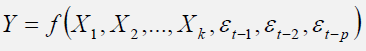
Another test for autocorrelation is the Breusch-Godfrey test, where for a regression function in the form of

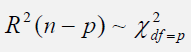
You estimate this regression equation and obtain its errors  t. Then, run the secondary regression function in the form of

To obtain the R-squared value and test it against a null hypothesis of no autocorrelation versus an alternate hypothesis of autocorrelation, where the test statistic follows a Chi-Square distribution of p degrees of freedom:

Fixing autocorrelation requires more advanced econometric models including the applications of ARIMA (Auto Regressive Integrated Moving Average) or ECM (Error Correction Models). However, one simple fix is to take the lags of the dependent variable for the appropriate periods, add them into the regression function, and test for their significance.