Detrending and Deseasonalizing

• By Admin
• November 12, 2014
• Comments Off on Detrending and Deseasonalizing

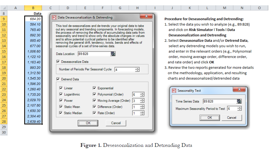
The data deseasonalization and detrending tool removes any seasonal and trending components in your original data (Figure 1). In forecasting models, the process usually includes removing the effects of accumulating datasets from seasonality and trend to show only the absolute changes in values and to allow potential cyclical patterns to be identified after removing the general drift, tendency, twists, bends, and effects of seasonal cycles of a set of time-series data. For example, a detrended dataset may be necessary to see a more accurate account of a company’s sales in a given year more clearly by shifting the entire dataset from a slope to a flat surface to better expose the underlying cycles and fluctuations.

Many time-series data exhibit seasonality where certain events repeat themselves after some time period or seasonality period (e.g., ski resorts’ revenues are higher in winter than in summer, and this predictable cycle will repeat itself every winter). Seasonality periods represent how many periods would have to pass before the cycle repeats itself (e.g., 24 hours in a day, 12 months in a year, 4 quarters in a year, 60 minutes in an hour, etc.). For deseasonalized and detrended data, a seasonal index greater than 1 indicates a high period or peak within the seasonal cycle, and a value below 1 indicates a dip in the cycle.

Procedure (Deseasonalization and Detrending)

• Select the data you wish to analyze (e.g., B9:B28) and click on Risk Simulator | Tools | Data Deseasonalization and Detrending.
• Select Deseasonalize Data and/or Detrend Data, select any detrending models you wish to run, enter in the relevant orders (e.g., polynomial order, moving average order, difference order, and rate order), and click OK.
• Review the two reports generated for more details on the methodology and application, and resulting charts and deseasonalized/detrended data.

Procedure (Seasonality Test)

• Select the data you wish to analyze (e.g., B9:B28) and click on Risk Simulator | Tools | Data Seasonality Test.
• Enter in the maximum seasonality period to test. That is, if you enter 6, the tool will test the following seasonality periods: 1, 2, 3, 4, 5, and 6. Period 1, of course, implies no seasonality in the data.
• Review the report generated for more details on the methodology and application, and resulting charts and seasonality test results. The best seasonality periodicity is listed first (ranked by the lowest RMSE error measure), and all the relevant error measurements are included for comparison: root mean squared error (RMSE), mean squared error (MSE), mean absolute deviation (MAD), and mean absolute percentage error (MAPE).