Distributional Analysis Tool

• By Admin
• October 28, 2014
• Comments Off on Distributional Analysis Tool

The distributional analysis tool is a statistical probability tool in Risk Simulator that is rather useful in a variety of settings. It can be used to compute the probability density function (PDF), which is also called the probability mass function (PMF), for discrete distributions (these terms are used interchangeably), where given some distribution and its parameters, we can determine the probability of occurrence given some outcome x. In addition, the cumulative distribution function (CDF) can be computed, which is the sum of the PDF values up to this x value. Finally, the inverse cumulative distribution function (ICDF) is used to compute the value x given the cumulative probability of occurrence. Example uses of PDF, CDF, and ICDF are provided herein.

This tool is accessible via Risk Simulator | Tools | Distributional Analysis. As an example of its use, Figure 1 shows the computation of a binomial distribution (i.e., a distribution with two outcomes, such as the tossing of a coin, where the outcome is either Head or Tail, with some prescribed probability of heads and tails). Suppose we toss a coin two times and set the outcome Head as a success. We use the binomial distribution with Trials = 2 (tossing the coin twice) and Probability = 0.50 (the probability of success, of getting Heads). Selecting the PDF and setting the range of values x as from 0 to 2 with a step size of 1 (this means we are requesting the values 0, 1, 2 for x), the resulting probabilities are provided in the table and in a graphic format, as well as the theoretical four moments of the distribution. As the possible

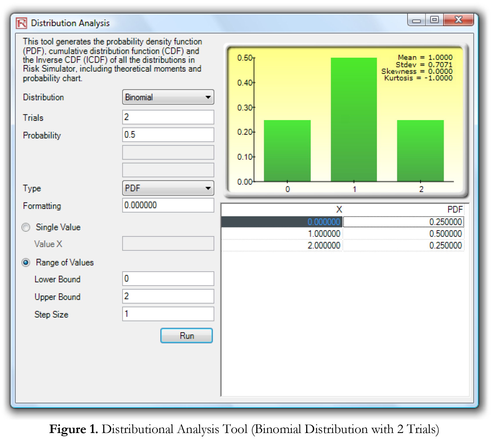
outcomes of the coin toss are Heads-Heads, Tails-Tails, Heads-Tails, and Tails-Heads, the probability of getting exactly no Heads is 25 percent, of getting one Head is 50 percent, and of getting two Heads is 25 percent. Similarly, we can obtain the exact probabilities of tossing the coin, say 20 times, as seen in Figure 2. The results are again presented both in tabular and graphic formats.

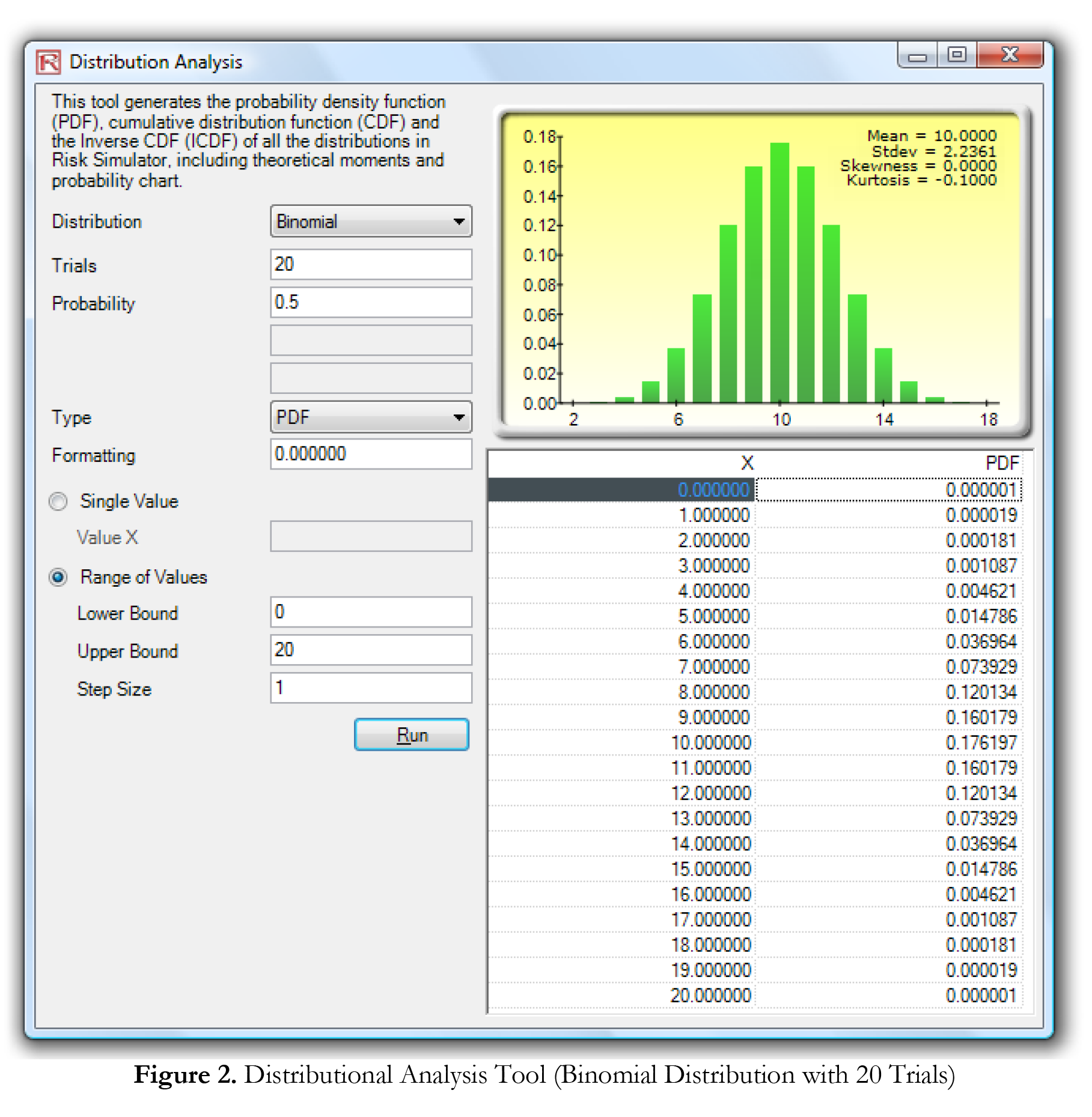
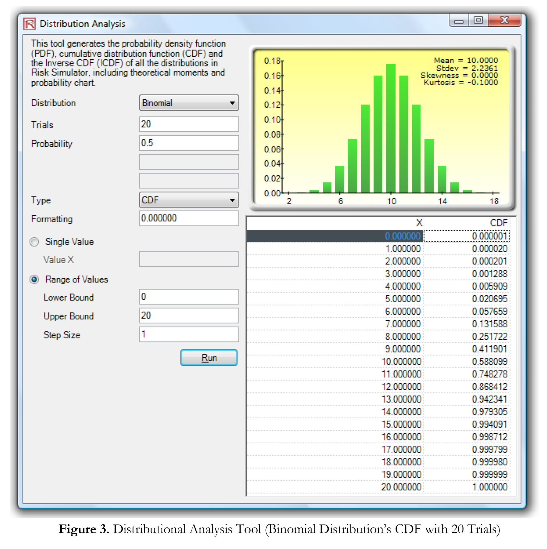
Figure 3 shows the same binomial distribution but now the CDF is computed. The CDF is simply the sum of the PDF values up to the point x. For instance, in Figure 2, we see that the probabilities of 0, 1, and 2 are 0.000001, 0.000019, and 0.000181, whose sum is 0.000201, which is the value of the CDF at x = 2 in Figure 3. Whereas the PDF computes the probabilities of getting exactly 2 heads, the CDF computes the probability of getting no more than 2 heads or up to 2 heads (or probabilities of 0, 1, and 2 heads). Taking the complement (i.e., 1 – 0.00021) obtains 0.999799, or 99.9799%, which is the probability of getting at least 3 heads or more.

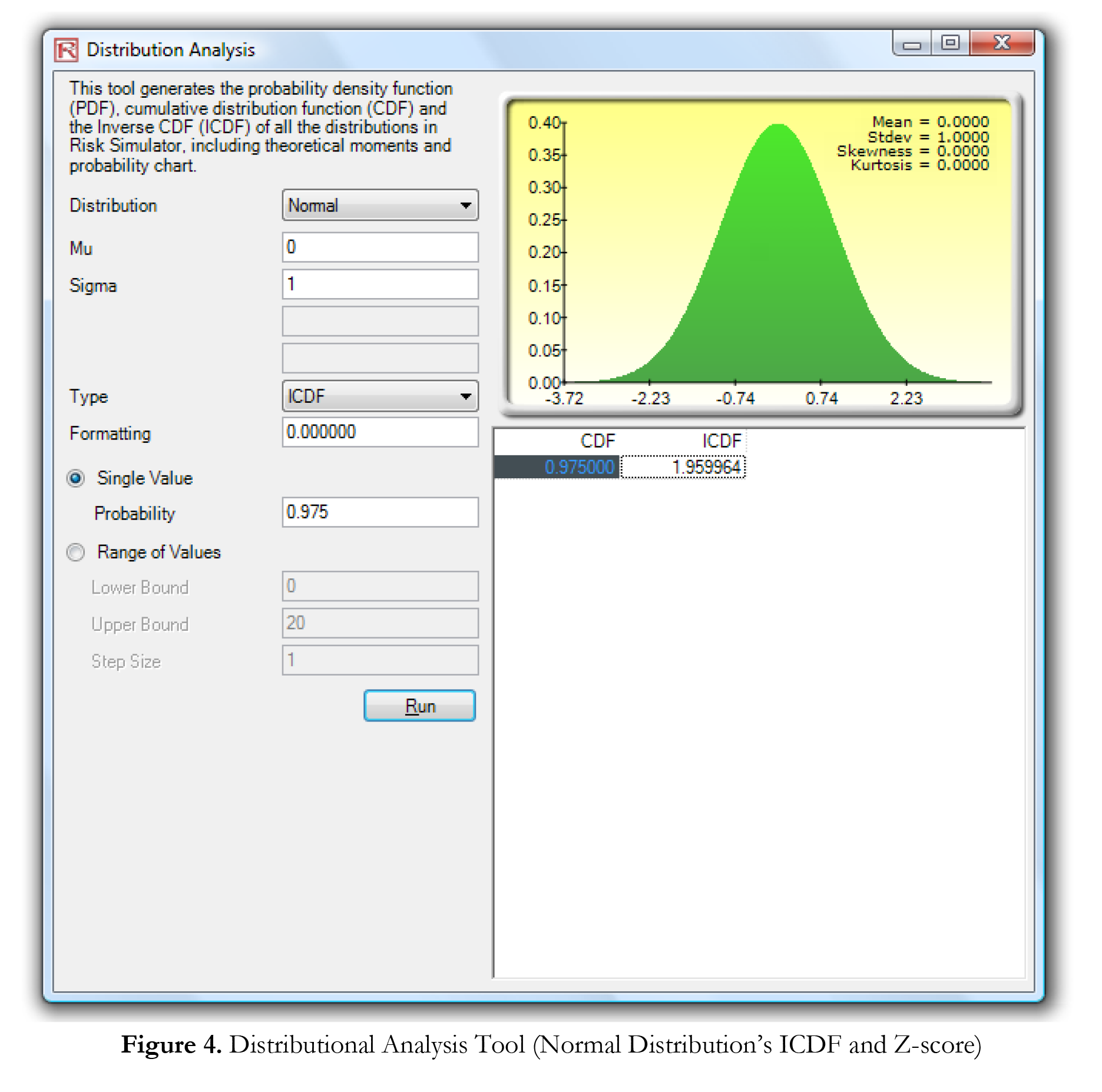
Using this distributional analysis tool, distributions even more advanced can be analyzed, such as the gamma, beta,
negative binomial, and many others in Risk Simulator. As further example of the tool’s use in a continuous distribution and the ICDF functionality, Figure 4 shows the standard normal distribution (normal distribution with a mean or mu of zero and standard deviation or sigma of one), where we apply the ICDF to find the value of x that corresponds to the cumulative probability of 97.50% (CDF). That is, a one-tail CDF of 97.50% is equivalent to a two-tail 95% confidence interval (there is a 2.50% probability in the right tail and 2.50% in the left tail, leaving 95% in the center or confidence interval area, which is equivalent to a 97.50% area for one tail). The result is the familiar Z-Score of 1.96. Therefore, using this distributional analysis tool, the standardized scores for other distributions and the exact and cumulative probabilities of other distributions can all be obtained quickly and easily.