Distributional Fitting and Goodness-of-Fit Tests

• By Admin
• October 28, 2014
• Comments Off on Distributional Fitting and Goodness-of-Fit Tests

Several statistical tests exist for deciding if a sample set of data comes from a specific distribution. The most commonly used are the Kolmogorov-Smirnov test and the Chi-Square test. Each test has its advantages and disadvantages. The following sections detail the specifics of these two tests as applied in distributional fitting in Monte Carlo simulation analysis. Other tests such as the Anderson-Darling, Jacque-Bera, and Wilkes-Shapiro are not used in Risk Simulator as these are parametric tests and their accuracy depends on the dataset being normal or near-normal. Therefore, these tests oftentimes yield suspect or inconsistent results.

Kolmogorov-Smirnov Test
The Kolmogorov-Smirnov (KS) test is based on the empirical distribution function of a sample dataset and belongs to a class of nonparametric tests. Nonparametric simply means no predefined distributional parameters are required. This nonparametric characteristic is the key to understanding the KS test, because it means that the distribution of the KS test statistic does not depend on the underlying cumulative distribution function being tested. In other words, the KS test is applicable across a multitude of underlying distributions. Another advantage is that it is an exact test as compared to the Chi-Square test, which depends on an adequate sample size for the approximations to be valid. Despite these advantages, the KS test has several important limitations: It only applies to continuous distributions, and it tends to be more sensitive near the center of the distribution than at the distribution’s tails. Also, the distribution must be fully specified.

Given N ordered data points Y1, Y2, … YN, the empirical distribution function is defined as Error! Objects cannot be created from editing field codes., where ni is the number of points less than Yi where Yi are ordered from the smallest to the largest value. This is a step function that increases by 1/N at the value of each ordered data point.

The null hypothesis is such that the dataset follows a specified distribution while the alternate hypothesis is that the dataset does not follow the specified distribution. The hypothesis is tested using the KS statistic defined as
Error! Objects cannot be created from editing field codes.
where F is the theoretical cumulative distribution of the continuous distribution being tested that must be fully specified (i.e., the location, scale, and shape parameters cannot be estimated from the data).

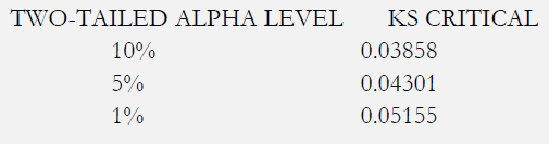
The hypothesis regarding the distributional form is rejected if the test statistic, KS, is greater than the critical value obtained from the table below. Notice that 0.03 to 0.05 are the most common levels of critical values (at the 1%, 5%, and 10% significance levels). Thus, any calculated KS statistic less than these critical values implies that the null hypothesis is not rejected and that the distribution is a good fit. There are several variations of these tables that use somewhat different scaling for the KS test statistic and critical regions. These alternative formulations should be equivalent, but it is necessary to ensure that the test statistic is calculated in a way that is consistent with how the critical values were tabulated. However, the rule of thumb is that a KS test statistic less than 0.03 or 0.05 indicates a good fit.

Chi-Square Test
The Chi-Square (CS) goodness-of-fit test is applied to binned data (i.e., data put into classes), and an attractive feature of the CS test is that it can be applied to any univariate distribution for which you can calculate the cumulative distribution function. However, the values of the CS test statistic are dependent on how the data are binned, and the test requires a sufficient sample size in order for the CS approximation to be valid. This test is sensitive to the choice of bins. The test can be applied to discrete distributions such as the binomial and the Poisson, while the KS test is restricted to continuous distributions.

The null hypothesis is such that the dataset follows a specified distribution while the alternate hypothesis is that the dataset does not follow the specified distribution. The hypothesis is tested using the CS statistic defined as

Error! Objects cannot be created from editing field codes.

where Oi is the observed frequency for bin i and Ei is the expected frequency for bin i. The expected frequency is calculated by Error! Objects cannot be created from editing field codes., where F is the cumulative distribution function for the distribution being tested, YU is the upper limit for class i, YL is the lower limit for class i, and N is the sample size.

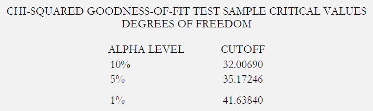
The test statistic follows a CS distribution with (k – c) degrees of freedom, where k is the number of nonempty cells and c is the number of estimated parameters (including location and scale parameters and shape parameters) for the distribution + 1. For example, for a three-parameter Weibull distribution, c = 4. Therefore, the hypothesis that the data are from a population with the specified distribution is rejected if Error! Objects cannot be created from editing field codes. where Error! Objects cannot be created from editing field codes. is the CS percent point function with k – c degrees of freedom and a significance level of α. Again, as the null hypothesis is such that the data follow some specified distribution, when applied to distributional fitting in Risk Simulator, a low p-value (e.g., less than 0.10, 0.05, or 0.01) indicates a bad fit (the null hypothesis is rejected) while a high p-value indicates a statistically good fit.