Dynamic Simulated Decision Trees

• By Admin
• February 4, 2015
• Comments Off on Dynamic Simulated Decision Trees

One major misunderstanding that analysts tend to have about real options is that they can be solved using decision trees alone. This is untrue. Instead, decision trees are a great way of depicting strategic pathways that a firm can take, showing graphically a decision road map of management’s strategic initiatives and opportunities over time. However, to solve a real options problem, it is better to combine decision‐tree analytics with real options analytics, rather than solely relying on decision trees. When used in framing real options,these trees should be more appropriately called strategy trees (used to define optimal strategic pathways).

Multiple other real options problems using more advanced techniques are required in certain circumstances. These models include the applications of stochastic optimization as well as other exotic types of options. In addition, as discussed, decision trees are insufficient when trying to solve real options problems because subjective probabilities with Bayesian updating are required as well as different discount rates at each node. The difficulties in forecasting the relevant discount rates and probabilities of occurrence are compounded over time, and the resulting values are oftentimes in error. However,decision trees by themselves are great as a depiction of management’s strategic initiatives and opportunities over time. Decision trees should be used in conjunction with real options analytics in more complex cases.

Models used to solve decision tree problems range from a simple expected value to more sophisticated Bayesian probability updating approaches. Neither of these approaches alone is applicable when trying to solve a real options problem. In addition, binomial lattices are a much better way to solve real options problems, and because these lattices can also ultimately be converted into decision trees, they are far superior to using decision trees as a stand‐alone application for real options. Nonetheless, there is a common ground between decision trees and real options analytics.

For instance, if a decision‐tree analysis is used (which by itself is insufficient for solving real options),then different discount rates have to be estimated at each decision node at different times because different projects at different times have different risk structures. Estimation errors will then be compounded on a large decision‐tree analysis. Binomial lattices using risk‐neutral probabilities avoid this error.In addition, risk‐free rates are objective and easy to obtain, and because volatility is obtained from a robust Monte Carlo simulation approach, the imputed risk‐neutral probability is more accurate, compared to guessing at the discount rate. Also, the discount rate requires a market benchmark that may or may not exist in the real options world (e.g., the beta coefficient is covariance divided by the variance of an external comparable market, to compute the CAPM discount rate).

One major conclusion that can be drawn using binomial lattices is that because risk‐adjusting cash flows provides the same results as risk‐adjusting the probabilities leading to those cash flows, the results stemming from a discounted cash flow analysis are identical to those generated using a binomial lattice. The only condition that is required is that the volatility of the cash flows be zero—in other words, the cash flows are assumed to be known with certainty. Because zero uncertainty exists, there is zero strategic option value, meaning that the net present value of a project is identical to its expanded net present value.

One of the fatal errors analysts tend to run into includes creating a decision tree and calculating the expected value using risk‐neutral probabilities, akin to the risk‐neutral probability used in binomial lattices. This approach is incorrect because risk‐neutral probabilities are calculated based on a constant volatility. The risk structures of nodes on a decision tree (for instance, e‐learning versus a dot.com strategy have very different risks and volatilities). In addition, for risk‐neutral probabilities, a Martingale process is required. That is, in a binomial lattice, each node has two bifurcations, an up and a down. The up and down jump sizes are identical in magnitude for a recombining lattice. This characteristic has to hold before risk‐neutral probabilities are valid. Clearly the return magnitudes of different events along the decision tree are different, and risk neutralization does not work here. Because risk‐neutral probabilities cannot be used, the risk‐free rate, therefore,cannot be used here for discounting the cash flows.Also, because risks are different at each strategy node, the market risk‐adjusted discount rate, such as a WACC, should also be different at every node.A correct single discount rate is difficult enough to calculate, let alone multiple discount rates on a complex tree, and the errors tend to compound by the time the NPV of the strategy is calculated.

In addition, chance nodes are usually added in decision‐tree analysis, indicating that a certain event may occur given a specific probability. For instance, chance nodes may indicate a 30 percent chance of a great economy, a 45 percent chance of a nominal one, and a 25 percent chance of a downturn.Then events and payoffs are associated with these chances. Back‐calculating these nodes using risk‐neutral probabilities will be incorrect because these are chance nodes, not strategic options. Because these three events are complementary––that is, their respective probabilities add up to 100 percent––one of these events must occur, and given enough trials, all of these events must occur at one time or another. Real options analysis stipulates that one does not know what will occur, but only what the strategic alternatives are if a certain event occurs. If chance nodes are required in an analysis, the discounted cash flow model can accommodate them to calculate an expected value, which could then be simulated based on the probability and distributional assumptions.These simulated values can then be run in a real options modeling environment.The results can be shown on a strategy tree looking similar to a decision tree as depicted in Chapter 13 of Modeling Risk (3rd Edition).However, strategic decision pathways should be shown in the strategy tree environment, and each strategy node or combinations of strategy nodes can be evaluated in the context of real options analysis as described throughout the chapter described. Then the results can be displayed in the strategy tree.

In summary, decision‐tree analysis is incomplete as a stand‐alone analysis in complex situations. Both the decision‐tree and real options methodologies discussed approach the same problem from different perspectives. However, a common ground could be reached.Taking the advantages of both approaches and melding them into an overall valuation strategy, decision trees should be used to frame the problem,real options analytics should be used to solve any existing strategic optionalities (either by pruning the decision tree into subtrees or solving the entire strategy tree at once), and the results should be presented back on a decision tree.These so‐called option strategy trees are useful for determining the optimal decision paths the firm should take.

ROV Decision Tree Module

Having made the preceding caveats on decision trees, know that they are still useful in a variety of settings especially when advanced analytics such as Integrated Risk Management is integrated into decision trees as presented in this section. Selecting Risk Simulator|ROV Decision Tree runs the Decision Tree module (Figure 1). ROV Decision Tree is used to create and value decision tree models. Additional advanced methodologies and analytics are also included:

• Decision Tree Models
• Monte Carlo Risk Simulation
• Sensitivity Analysis
• Scenario Analysis
• Bayesian (Joint and Posterior Probability Updating)
• Expected Value of Information
• MINIMAX
• MAXIMIN
• Risk Profiles

Example Case Illustration

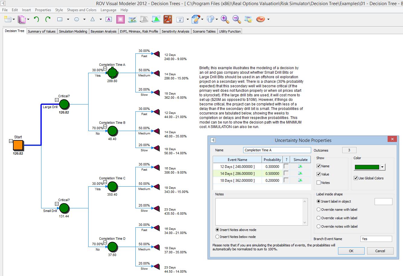
Figure 1, a sample oil and gas drilling project, illustrates the modeling of a risky decision on whether small drill bits or large drill bits should be used in an offshore oil exploration project on a secondary well Start
the ROV Decision Tree and click on File| Example| 01 Basic Large or Small Development to load this example to follow along.

In the example, there is an expected 30% probability that this secondary well will become critical (if the primary well does not function properly or when oil prices start to skyrocket), or 70% probability (its complement) that it will not. If the large drill bits are used, it will cost more to set up (e.g., $20M as opposed to $10M). However, if things do become critical, the project can be completed with less of a delay if a large initial drill bit is used rather than a small drill bit. The event probabilities, weeks to completion or delays,and their respective probabilities of delays are mapped in the decision tree. This model can be then be
run to show the decision path with the minimum cost, and a risk simulation can also be run and the results
can be tabulated as a probability distribution (Figure 2).The following provides more details on how the
decision is set up as well as what each of the nodes and values represent:

• Start by drawing the entire decision tree, then add the values after the tree has been constructed.
• Squares are decision nodes (i.e., a decision that has to be made) where in the example, we see that the decision is whether to use a small drill bit or a large drill bit.
• Circles are uncertainty nodes where various events can occur and each event carries with it some probability, and the sum of the probabilities in each circle uncertainty node must sum to 100%.
• Finally, the decision tree must always end on the right with the triangular terminal nodes. A
  decision tree cannot be modeled and solved unless every final node is a terminal node.
• The decision tree implementation pathway and sequence of events progress from the left to right.In the example, we see that the decision (the initial square decision node) is whether to implement the large drill bit or small drill bit. The decision takes two outcome paths: small or large drill bits.
• Regardless of which decision path is taken, there is uncertainty in terms of whether the secondary well will become critical (30% probability) or not critical (70% probability). This uncertainty is independent of and applies whether the large or small drills are implemented, which is why you see the two circular uncertainty nodes in the second step in the figure, denoted as “Critical?” The two identical nodes splits into two outcomes: “Yes” it is critical (30%) and “No” it is not critical (70%), as depicted as the third column of the decision tree.
• Next, the level of uncertainty is the secondary well completion time. Although the well will be completed faster with the larger drill bit and slower with the smaller drill bit, the completion time is still uncertain. With the large drill bit, regardless of whether the well is critical or not, the uncertainty in terms of completion time can be 12 days with a 30% probability, 14 days with a 50% probability, and 18 days with 20% probability. Note that this uncertainty node has three outcomes, and the sum of the probabilities for the uncertainty node must equal 100%. This Completion Time A node is replicated for Completion Time B node as the time to complete the wells, again, are independent of whether the well is critical or not, although it is dependent on the drill size. This is why in Completion Time C and D, which are identical, have 16 days, 18 days, and 23 days, indicating a delay in completion time when the small drill bit is used.
• Finally, each of the branches on the right must finish with triangular terminal nodes. These nodes will require user inputs in the payoff under each situation. In other words, if the large drill bit is executed and the well is critical, and if the well could somehow be completed in 12 days, the present value of the cost or payoff is a cost of $248M. Continue with the terminal nodes and complete the inputs for the cost structure.
• Note that you can enter the terminal values as either positive or negative, and terminal nodes are usually net present values or costs (although other variables can be used, of course, such as time or resources).Since we are modeling the cost, when we run the analysis, select the cost Minimization Option.If these payoffs are net present values, then by all means choose the Maximum Payoff option.
• As mentioned, finish drawing the decision tree from left to right first, then start entering the values in the nodes, either left to right or right to left, it really does not matter. The following are the required inputs in the sample decision tree:
• All terminal node payoffs. As explained, in this example, the payoffs are the costs under each pathway, for example, $248M, $286M, $362M, and so forth. You can double‐click on the each of the terminal nodes to enter the required inputs.
  All probabilities of the event outcomes in the uncertainty nodes. For instance, doubleclick on the circle uncertainty nodes and enter the probabilities of each event branch. In the Critical node, enter 30% and 70%. In the Completion Time nodes, enter the 30%, 50%, and 20% probabilities. Again, all probabilities in the same node must sum to 100%.
• Then, click on the Run icon and select either Minimize or Maximize. In this example where we use cost as the positive payoff values, Minimize is the correct option. After running, you will see a few things:
• The optimal path will be highlighted. In this case, the minimal cost is to execute the large drill, which will, given the cost structure and probability of various event outcomes, be the course of action that best minimizes the total cost to the company. Note that the highlighted path is short in this case as there is only one decision node, and the highlighted path shows which decision to take. The path will not continue past any uncertainty nodes because these are uncertain outcomes and, hence, the model will not be able to determine which event outcome or path will occur. In larger decision trees with additional decision nodes, you will see a longer highlighted optimal path.
  Additional values are now displayed on the decision tree.
• In the terminal node, you will see the percentages, such as 9.00% for the first terminal node. This is the expected probability given this pathway, assuming independence among the probabilistic outcomes.That is, 30% × 30% = 9.00%. The first 30% is the Critical = Yes path, and the second 30% is the Fast Completion Time path.As another example, the second terminal node is 15.00%, which is computed by multiplying 30% × 50% = 15.00% (the Critical = Yes and Completion Time = Medium path). All other percentages are computed in a similar fashion.
• Under each uncertainty node you will now see a computed number. These are the expectation values. For instance, the value $289.80 under the Completion Time A node is computed by 30% × $248 + 50% × $286 + 20% × $362 = $289.80.The same expected value calculation applies to the other circular uncertainty nodes.
• Finally, you see the initial square decision node shows a computed value of $120.82, which is the minimum value comparing $120.82 and $131.44. The highlighted path indicates the best decision to take, and in this case it is to go with the large drill bit, which will minimize the total expected cost of the project.
• Users can click on the Summary of Values tab to see a tabular outcome of the values discussed above.
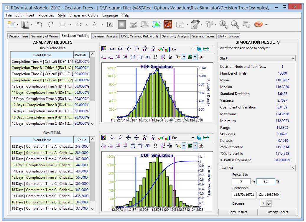
• In the Simulation Modeling tab, the decision node’s simulated results will be seen (Figure 2):
• The simulated mean value is $118.39 for the cost, close to the single‐point estimated cost of $120.82 in the decision tree. The simulated mean value includes all the assumptions that we set up in the model.
• Note that only user input values can be simulated, which means only the terminal payoff values and the uncertainty probability values can be set as input assumptions for the simulation to proceed.
• Figure 1 shows a sample user interface that opens when one of the uncertainty nodes is double‐clicked. Here you see that the set input assumption icon can be clicked under the column named Simulate. In this column, users can set simple probability assumptions or create their own equations to simulate.
• The simulated result in Figure 2 shows that the 90% confidence interval (i.e., 5% on the left tail and 5% on the right tail with 90% in the middle of the distribution, which is the same as entering the 5th and 95th Percentiles) returns a value of $115.70M and $121.12M. In the 5% best‐case scenario, the cost will be under $115M, whereas it will be over $121M in the worst‐case scenario.
• 

  

  The following are some key quick getting started tips and procedures for using this intuitive tool:

• There are 11 localized languages available in this module and the current language can be changed through the Language menu. Select the language of your choice to begin; English is the default language selected.
• Insert Option nodes or Insert Terminal nodes by first selecting any existing node and then clicking on
  the option node icon (square) or terminal node icon (triangle), or use the functions in the Insert menu.
• Modify individual Option Node or Terminal Node properties by double‐clicking on a node. Sometimes when you click on a node, all subsequent child nodes are also selected (this allows you to move the entire tree starting from that selected node). If you wish to select only that node, you may have to click on the empty background and click back on that node to select it individually. Also, you can move individual nodes or the entire tree started from the selected node depending on the current setting (right‐click, or in the Edit menu, and select Move Nodes Individually or Move Nodes Together).
• The following are some quick descriptions of the things that can be customized and configured in the node properties user interface. It is simplest to try different settings for each of the following to see its effects in the Strategy Tree:
• • Name. Name shown above the node.
  • Value. Value shown below the node.
  • Excel Link. Links the value from an Excel spreadsheet’s cell.
  • Notes. Notes can be inserted above or below a node.
  • Show in Model. Show any combinations of Name, Value, and Notes.
  • Local Color versus Global Color. Node colors can be changed locally to a node or globally.
  • Label Inside Shape. Text can be placed inside the node (you may need to make the node wider to accommodate longer text).
  • Branch Event Name. Text can be placed on the branch leading to the node to indicate the event leading to this node.
  • Select Real Options. A specific real option type can be assigned to the current node. Assigning real options to nodes allows the tool to generate a list of required input variables.
• Global Elements are all customizable, including elements of the Strategy Tree’s Background, Connection
  Lines, Option Nodes, Terminal Nodes, and Text Boxes. For instance, the following settings can be changed for each of the elements:
• • Font settings on Name, Value, Notes, Label, Event names.
  • Node Size (minimum and maximum height and width).
  • Borders (line styles, width, and color).
  • Shadow (colors and whether to apply a shadow or not).
  • Global Color.
  • Global Shape
• The Edit menu’s View Data Requirements Window command opens a docked window on the right of the Strategy Tree such that when an option node or terminal node is selected, the properties of that node will be displayed and can be updated directly.This feature provides an alternative to doubleclicking on a node each time.
• Example Files are available in the File menu to help you get started on building Decision Trees and
  Strategy Trees
• Protect File from the File menu allows the Strategy Tree to be encrypted with up to a 256‐bit password
  encryption. Be careful when a file is being encrypted because if the password is lost, the file can no longer be opened.
• Capturing the Screen or printing the existing model can be done through the File menu. The captured screen can then be pasted into other software applications.
• Add, Duplicate, Rename, and Delete a Strategy Tree can be performed through right‐clicking the Strategy Tree tab or the Edit menu.
• You can also Insert File Link and Insert Comment on any option or terminal node, or Insert Text or Insert Picture anywhere in the background or drawing canvas area.
• You can Change Existing Styles, or Manage and Create Custom Styles of your Strategy Tree (this includes
  size, shape, color schemes, and font size/color specifications of the entire Strategy Tree).
• Insert Decision, Insert Uncertainty, or Insert Terminal nodes by selecting any existing node and then
  clicking on the decision node icon (square), uncertainty node icon (circle), or terminal node icon (triangle), or use the functionalities in the Insert menu.
• Modify individual Decision, Uncertainty, or Terminal nodes’ properties by double‐clicking on a node. The following are some additional unique items in the Decision Tree module that can be customized and configured in the node properties user interface:
• • Decision Nodes: Custom Override or Auto Compute the value on a node. The automatically compute option is set as default and when you click RUN on a completed Decision Tree model, the decision nodes will be updated with the results.
  • Uncertainty Nodes: Event Names, Probabilities, and Set Simulation Assumptions. You can add probability event names, probabilities, and simulation assumptions only after the uncertainty branches are created.
  • Terminal Nodes: Manual Input, Excel Link, and Set Simulation Assumptions. The terminal event payoffs can be entered manually or linked to an Excel cell (e.g., if you have a large Excel model that computes the payoff, you can link the model to this Excel model’s output cell) or set probability distributional assumptions for running simulations.
• View Node Properties Window is available from the Edit menu and the selected node’s properties will
  update when a node is selected
• The Decision Tree module also comes with the following advanced analytics:
• • Monte Carlo Risk Simulation Modeling on Decision Trees
  • Bayes Analysis for obtaining posterior probabilities
  • Expected Value of Perfect Information, MINIMAX and MAXIMIN Analysis, Risk Profiles, and Value of Imperfect Information
  • Sensitivity Analysis
  • Scenario Analysis
  • Utility Function Analysis

  Simulating a Decision Tree
  This tool runs Monte Carlo risk simulation on the decision tree (Figure 2). It allows you to set probability
  distributions as input assumptions for running simulations. You can either set an assumption for the selected node or set a new assumption and use this new assumption (or use previously created assumptions) in a numerical equation or formula. For example, you can set a new assumption called Normal (e.g., normal distribution with a mean of 100 and standard deviation of 10) and run a simulation in the decision tree, or use this assumption in an equation such as (100*Normal+15.25).

  Create your own model in the numerical expression box. You can use basic computations or add existing variables into your equation by double‐clicking on the list of existing variables. New variables can be added to the list as required either as numerical expressions or assumptions.

  Bayes Analysis on Decision Trees

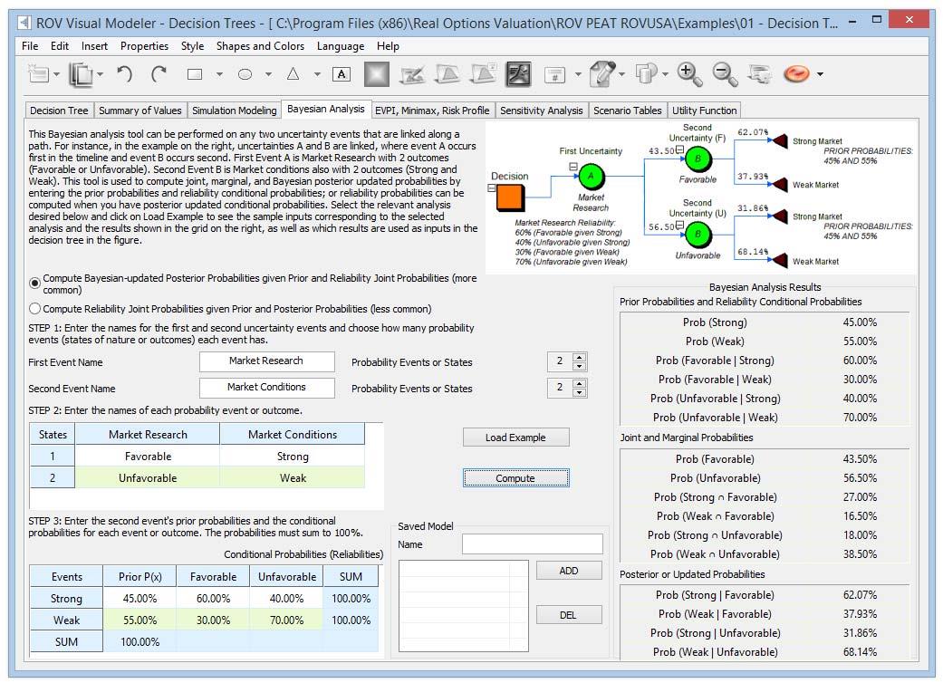
  This Bayesian analysis tool (Figure 3) can be used on any two uncertainty events that are linked along a
  path. For instance, in the example on the right in Figure 3, uncertainties A and B are linked, where event
  A occurs first in the timeline and event B occurs second. First Event A is Market Research with 2 outcomes
  (Favorable or Unfavorable). Second Event B is Market Conditions also with 2 outcomes (Strong and Weak). This tool is used to compute joint, marginal, and Bayesian posterior‐updated probabilities by entering the prior probabilities and reliability conditional probabilities; or reliability probabilities can be computed when you have posterior‐updated conditional probabilities. Select the relevant analysis desired and click on Load Example to see the sample inputs corresponding to the selected analysis and the results shown in the grid on the right, as well as which results are used as inputs in the decision tree in Figure 3.

  Procedure

• Enter the names for the first and second uncertainty events and choose how many probability events (states of nature or outcomes) each event has
• Enter the names of each probability event or outcome.
• Enter the second event’s prior probabilities and the conditional probabilities for each event or outcome.
  The probabilities must sum to 100%.
• Expected Value of Perfect Information, MINIMAX and MAXIMIN Analysis, Risk Profiles, and Value of Imperfect Information in Decision Trees

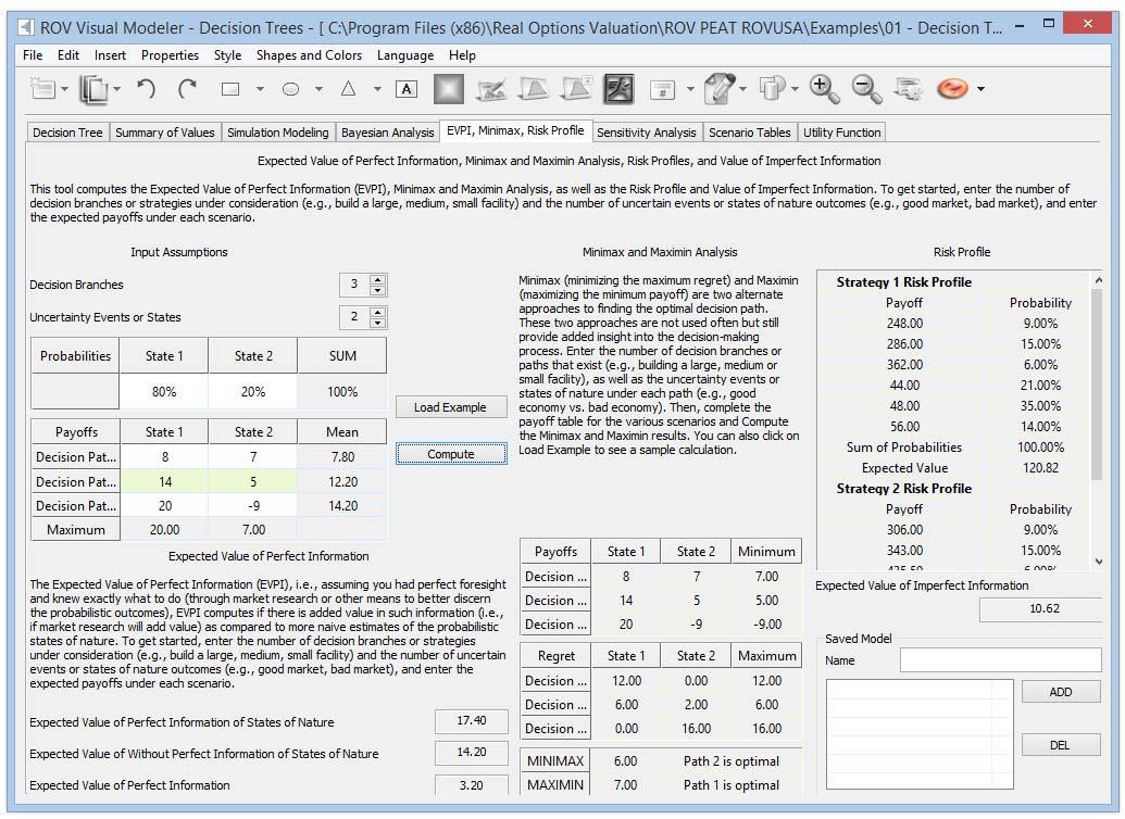
  This tool (Figure 4) computes the Expected Value of Perfect Information (EVPI), and MINIMAX and MAXIMIN Analysis, as well as the Risk Profile and the Value of Imperfect Information. To get started, enter the number of decision branches or strategies under consideration (e.g., build a large, medium, or small facility), the number of uncertain events or states of nature outcomes (e.g., good market, bad market), and the expected payoffs under each scenario.

  The Expected Value of Perfect Information (EVPI), that is, assuming you had perfect foresight and knew exactly what to do (through market research or other means to better discern the probabilistic outcomes), computes if there is added value in such information (i.e., if market research will add value) as compared to more naïve estimates of the probabilistic states of nature. To get started, enter the number of decision branches or strategies under consideration (e.g., build a large, medium, or small facility) and the number of uncertain events or states of nature outcomes (e.g., good market, bad market), and enter the expected payoffs under each scenario.

  MINIMAX (minimizing the maximum regret) and MAXIMIN (maximizing the minimum payoff) are two alternate approaches to finding the optimal decision path. These two approaches are not used often but still provide added insight into the decision‐making process. Enter the number of decision branches or paths that exist (e.g., build a large, medium, or small facility), as well as the uncertainty events or states of nature under each path (e.g., good economy vs. bad economy). Then, complete the payoff table for the various scenarios and Compute the MINIMAX and MAXIMIN results. You can also click on Load Example to see a sample calculation.

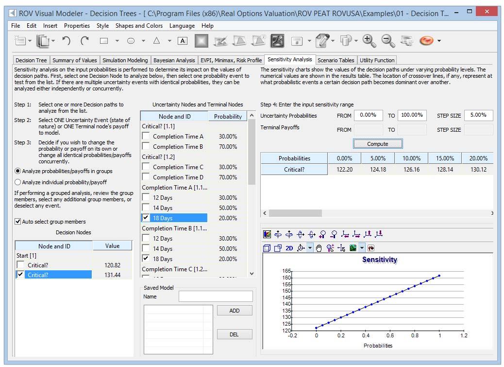
  Sensitivity Analysis in Decision Trees

  Sensitivity analysis (Figure 5) on the input probabilities is performed to determine the impact of inputs on the values of decision paths. First, select one Decision Node to analyze and then select one probability event to test from the list. If there are multiple uncertainty events with identical probabilities, they can be analyzed either independently or concurrently

  The sensitivity charts show the values of the decision paths under varying probability levels. The numerical values are shown in the results table. The location of crossover lines, if any, represents at what probabilistic events a certain decision path becomes dominant over another.

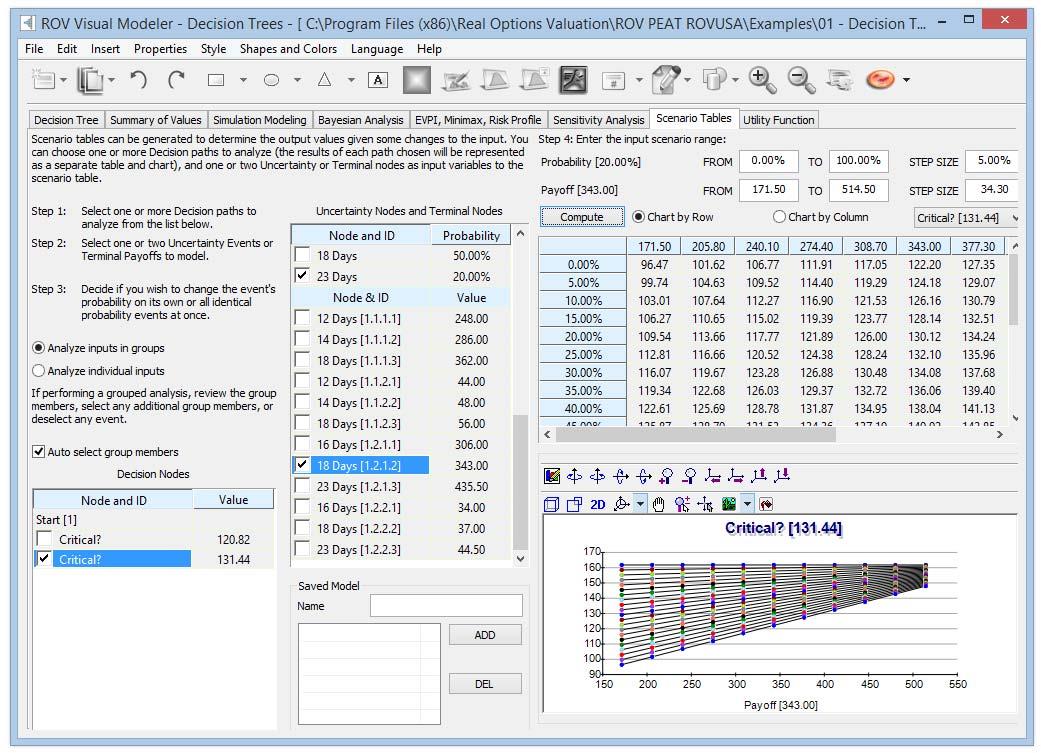
  Scenario Tables in Decision Trees

  Scenario tables (Figure 6) can be generated to determine the output values given some changes to the input. You can choose one or more Decision paths to analyze (the results of each path chosen will be represented as a separate table and chart) and one or two Uncertainty or Terminal nodes as input variables to the scenario table.

  Procedure

• Select one or more Decision paths to analyze from the list.
• Select one or two Uncertainty Events or Terminal Payoffs to model
• Decide if you wish to change the event’s probability on its own or all identical probability events at
  once.
• Enter the input scenario range.
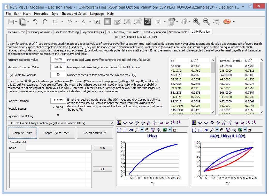
• Utility Functions in Decision Trees

  Utility functions (Figure 7), or U(x), are sometimes used in place of expected values of terminal payoffs in
  a decision tree. U(x) can be developed two ways: using tedious and detailed experimentation of every possible outcome or an exponential extrapolation method (used here). They can be modeled for a decision maker who is risk‐averse (downsides are more disastrous or painful than an equal upside potential), riskneutral (upsides and downsides have equal attractiveness), or risk‐loving (upside potential is more attractive). Enter the minimum and maximum expected value of your terminal payoffs and the number of data points in between to compute the utility curve and table.

  If you had a 50:50 gamble where you either earn $X or lose –$X/2 versus not playing and getting a $0 payoff, what would this $X be? For example, if you are indifferent between a bet where you can win $100 or lose –$50 with equal probability compared to not playing at all, then your X is $100. Enter the X in the Positive Earnings box. Note that the larger X is, the less risk‐averse you are, and whereas a smaller X indicates that you are more risk‐averse.

  Enter the required inputs, select the U(x) type, and click Compute Utility to obtain the results. You can also apply the computed U(x) values to the decision tree to rerun it, or revert the tree back to using expected values of the payoffs.