Multivariate Regression, Part 2

• By Admin
• November 24, 2014
• Comments Off on Multivariate Regression, Part 2

As noted in “Multivariate Regression, Part 1,” it is assumed that the user is knowledgeable about the fundamentals of regression analysis. In this part, we continue our coverage of the topic by examining stepwise regression and goodness-of-fit.

Stepwise Regression
One powerful automated approach to regression analysis is “stepwise regression” and based on its namesake, the regression process proceeds in multiple steps. There are several ways to set up these stepwise algorithms including the correlation approach, forward method, backward method, and the forward and backward method (these methods are all available in Risk Simulator).

In the correlation method, the dependent variable (Y) is correlated to all the independent variables (X), and starting with the X variable with the highest absolute correlation value, a regression is run, then subsequent X variables are added until the pvalues indicate that the new X variable is no longer statistically significant. This approach is quick and simple but does not account for interactions among variables, and an X variable, when added, will statistically overshadow other variables.

In the forward method, we first correlate Y with all X variables, run a regression for Y on the highest absolute value correlation of X, and obtain the fitting errors. Then, correlate these errors with the remaining X variables and choose the highest absolute value correlation among this remaining set and run another regression. Repeat the process until the p-value for the latest X variable coefficient is no longer statistically significant and then stop the process.

In the backward method, run a regression with Y on all X variables and reviewing each variable’s p-value, systematically eliminate the variable with the largest p-value, and then run a regression again, repeating each time until all p-values are statistically significant. In the forward and backward method, apply the forward method to obtain three X variables and then apply the backward approach to see if one of them needs to be eliminated because it is statistically insignificant. Then repeat the forward method, and then the backward method until all remaining X variables are considered.

Goodness-of-Fit
Goodness-of-fit statistics provide a glimpse into the accuracy and reliability of the estimated regression model. They usually take the form of a t-statistic, F-statistic, R-squared statistic, adjusted R-squared statistic, or Durbin-Watson statistic, and their respective probabilities. The following sections discuss some of the more common regression statistics and their interpretation.

The R-squared (R2), or coefficient of determination, is an error measurement that looks at the percent variation of the dependent variable that can be explained by the variation in the independent variable for a regression analysis. The coefficient of determination can be calculated by:

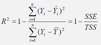
where the coefficient of determination is one less the ratio of the sums of squares of the errors (SSE) to the total sums of squares (TSS). In other words, the ratio of SSE to TSS is the unexplained portion of the analysis, thus, one less the ratio of SSE to TSS is the explained portion of the regression analysis.

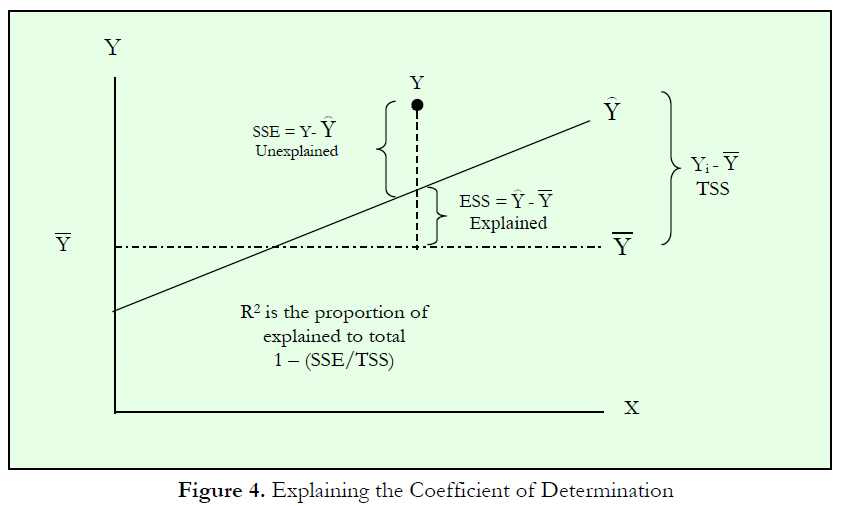
Figure 4 provides a graphical explanation of the coefficient of determination. The estimated regression line is characterized by a series of predicted values (Error! Objects cannot be created from editing field codes.); the average value of the dependent variable’s data points is denoted Error! Objects cannot be created from editing field codes.; and the individual data points are characterized by Yi. Therefore, the total sum of squares, that is, the total variation in the data or the total variation about the average dependent value, is the total of the difference between the individual dependent values and their average (seen as the total squared distance of Error! Objects cannot be created from editing field codes. in Figure 4).

The explained sum of squares, the portion that is captured by the regression analysis, is the total of the difference between the regression’s predicted value and the average dependent variable’s dataset (seen as the total squared distance of Error! Objects cannot be created from editing field codes. in Figure 4). The difference between the total variation (TSS) and the explained variation (ESS) is the unexplained sums of squares, also known as the sums of squares of the errors (SSE).

Another related statistic, the adjusted coefficient of determination, or the adjusted R-squared ( R 2 ), corrects for the number of independent variables (k) in a multivariate regression through a degrees of freedom correction to provide a more conservative estimate:

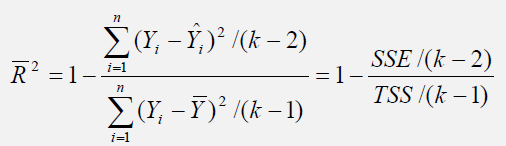
The adjusted R-squared should be used instead of the regular R-squared in multivariate regressions because every time an independent variable is added into the regression analysis, the R-squared will increase, indicating that the percent variation explained has increased. This increase occurs even when nonsensical regressors are added. The adjusted R-squared takes the added regressors into account and penalizes the regression accordingly, providing a much better estimate of a regression model’s goodness-of-fit.

Other goodness-of-fit statistics include the t-statistic and the F-statistic. The former is used to test if each of the estimated slope and intercept(s) is statistically significant, that is, if it is statistically significantly different from zero (therefore making sure that the intercept and slope estimates are statistically valid). The latter applies the same concepts but simultaneously for the entire regression equation including the intercept and slope(s).