Optimization Procedures: Continuous Optimization

• By Admin
• September 17, 2014
• Comments Off on Optimization Procedures: Continuous Optimization

Many algorithms exist to run optimization and many different procedures exist when optimization is coupled with Monte Carlo simulation. In Risk Simulator, there are three distinct optimization procedures and optimization types as well as different decision variable types. For instance, Risk Simulator can handle Continuous Decision Variables (1.2535, 0.2215, and so forth), Integer Decision Variables (e.g., 1, 2, 3, 4 or 1.5, 2.5, 3.5, and so forth), Binary Decision Variables (1 and 0 for go and no-go decisions), and Mixed Decision Variables (both integers and continuous variables). On top of that, Risk Simulator can handle Linear Optimization (i.e., when both the objective and constraints are all linear equations and functions) and Nonlinear Optimizations (i.e., when the objective and constraints are a mixture of linear and nonlinear functions and equations).

As far as the optimization process is concerned, Risk Simulator can be used to run a Discrete Optimization, that is, an optimization that is run on a discrete or static model, where no simulations are run. In other words, all the inputs in the model are static and unchanging. This optimization type is applicable when the model is assumed to be known and no uncertainties exist. Also, a discrete optimization can first be run to determine the optimal portfolio and its corresponding optimal allocation of decision variables before more advanced optimization procedures are applied. For instance, before running a stochastic optimization problem, a discrete optimization is first run to determine if solutions to the optimization problem exist before a more protracted analysis is performed.

Next, Dynamic Optimization is applied when Monte Carlo simulation is used together with optimization. Another name for such a procedure is Simulation-Optimization. That is, a simulation is first run, then the results of the simulation are applied in the Excel model, and then an optimization is applied to the simulated values. In other words, a simulation is run for N trials, and then an optimization process is run for M iterations until the optimal results are obtained or an infeasible set is found. Using Risk Simulator’s optimization module, you can choose which forecast and assumption statistics to use and replace in the model after the simulation is run. Then, these forecast statistics can be applied in the optimization process. This approach is useful when you have a large model with many interacting assumptions and forecasts, and when some of the forecast statistics are required in the optimization. For example, if the standard deviation of an assumption or forecast is required in the optimization model (e.g., computing the Sharpe Ratio in asset allocation and optimization problems where we have mean divided by standard deviation of the portfolio), then this approach should be used.

The Stochastic Optimization process, in contrast, is similar to the dynamic optimization procedure with the exception that the entire dynamic optimization process is repeated T times. That is, a simulation with N trials is run, and then an optimization is run with M iterations to obtain the optimal results. Then the process is replicated T times. The results will be a forecast chart of each decision variable with T values. In other words, a simulation is run and the forecast or assumption statistics are used in the optimization model to find the optimal allocation of decision variables. Then, another simulation is run, generating different forecast statistics, and these new updated values are then optimized, and so forth. Hence, the final decision variables will each have their own forecast chart, indicating the range of the optimal decision variables. For instance, instead of obtaining single-point estimates in the dynamic optimization procedure, you can now obtain a distribution of the decision variables and, hence, a range of optimal values for each decision variable, also known as a stochastic optimization.

Finally, an Efficient Frontier optimization procedure applies the concepts of marginal increments and shadow pricing in optimization. That is, what would happen to the results of the optimization if one of the constraints were relaxed slightly? Say for instance, the budget constraint is set at $1 million. What would happen to the portfolio’s outcome and optimal decisions if the constraint were now $1.5 million, or $2 million, and so forth. This is the concept of the Markowitz efficient frontier in investment finance, where if the portfolio standard deviation is allowed to increase slightly, we want to know what additional returns the portfolio will generate. This process is similar to the dynamic optimization process with the exception that one of the constraints is allowed to change, and with each change, the simulation and optimization process is run. This process is best applied manually using Risk Simulator. This process can be run either manually (rerunning the optimization several times) or automatically (using Risk Simulator’s changing constraint and efficient frontier functionality). As example, the manual process is: Run a dynamic or stochastic optimization, then rerun another optimization with a new constraint, and repeat that procedure several times. This manual process is important, as by changing the constraint, the analyst can determine if the results are similar or different and, hence, whether it is worthy of any additional analysis, or to determine how far a marginal increase in the constraint should be to obtain a significant change in the objective and decision variables. This is done by comparing the forecast distribution of each decision variable after running a stochastic optimization. Alternatively, the automated efficient frontier approach will be shown later.

One item is worthy of consideration. Other software products exist that supposedly perform stochastic optimization, but, in fact, they do not. For instance, after a simulation is run, then one iteration of the optimization process is generated, and then another simulation is run, then the second optimization iteration is generated and so forth. This process is simply a waste of time and resources; in optimization, the model is put through a rigorous set of algorithms, where multiple iterations (ranging from several to thousands) are required to obtain the optimal results. Hence, generating one iteration at a time is a waste of time and resources. The same portfolio can be solved in under a minute using Risk Simulator as compared to hours using such a backward approach. Also, such an approach will typically yield bad results and is not a stochastic optimization approach. Be extremely careful of such methodologies when applying optimization to your models.

The following are example optimization problems. One uses continuous decision variables while the other uses discrete integer decision variables. In either model, you can apply discrete optimization, dynamic optimization, or stochastic optimization, or even manually generate efficient frontiers with shadow pricing. Any of these approaches can be used for these examples. Therefore, for simplicity, only the model setup is illustrated and it is up to the user to decide which optimization process to run. Also, the continuous decision variable example uses the nonlinear optimization approach (because the portfolio risk computed is a nonlinear function, and the objective is a nonlinear function of portfolio returns divided by portfolio risks) while the second example of an integer optimization is an example of a linear optimization model (its objective and all of its constraints are linear). Therefore, these examples encapsulate all of the procedures aforementioned.

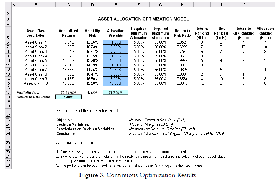
Figure 1 illustrates the sample continuous optimization model. The example uses the 11 Continuous Optimization file found on Risk Simulator | Example Models. It has 10 distinct asset classes (e.g., different types of mutual funds or stocks) where the idea is to most efficiently and effectively allocate the portfolio holdings, that is, to generate the best portfolio returns possible given the risks inherent in each asset class (best bang for the buck). To truly understand the concept of optimization, we must delve more deeply into this sample model to see how the optimization process can best be applied.

The model shows the 10 asset classes and each asset class has its own set of annualized returns and annualized volatilities. These return and risk measures are annualized values such that they can be consistently compared across different asset classes. Returns are computed using the geometric average of the relative returns while the risks are computed using the logarithmic relative stock returns approach.

The Allocation Weights in column E hold the decision variables, which are the variables that need to be tweaked and tested such that the total weight is constrained at 100% (cell E17). Typically, to start the optimization, we will set these cells to a uniform value, where in this case, cells E6 to E15 are set at 10% each. In addition, each decision variable may have specific restrictions in its allowed range. In this example, the lower and upper allocations allowed are 5% and 35%, as seen in columns F and G. This means that each asset class may have its own allocation boundaries. Next, column H shows the return to risk ratio, which is simply the return percentage divided by the risk percentage, where the higher this value, the bigger the bang for the buck. The remaining model shows the individual asset class rankings by returns, risk, return to risk ratio, and allocation. In other words, these rankings show at a glance which asset class has the lowest risk, or the highest return, and so forth.

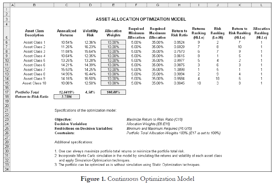
The portfolio’s total returns in cell C17 is SUMPRODUCT(C6:C15, E6:E15), that is, the sum of the allocation weights multiplied by the annualized returns for each asset class. In other words, we haveError! Objects cannot be created from editing field codes., where RP is the return on the portfolio, RA,B,C,D are the individual returns on the projects, and ωA,B,C,D are the respective weights or capital allocation across each project.
In addition, the portfolio’s diversified risk in cell D17 is computed by taking

Error! Objects cannot be created from editing field codes.

Here, ρi,j are the respective cross-correlations between the asset classes. Hence, if the cross-correlations are negative, there are risk diversification effects, and the portfolio risk decreases. However, to simplify the computations here, we assume zero correlations among the asset classes through this portfolio risk computation, but assume the correlations when applying simulation on the returns as will be seen later. Therefore, instead of applying static correlations among these different asset returns, we apply the correlations in the simulation assumptions themselves, creating a more dynamic relationship among the simulated return values.

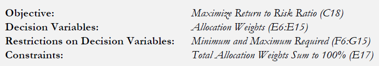
Finally, the return to risk ratio or Sharpe Ratio is computed for the portfolio. This value is seen in cell C18 and represents the objective to be maximized in this optimization exercise. To summarize, we have the following specifications in this example model:

Procedure

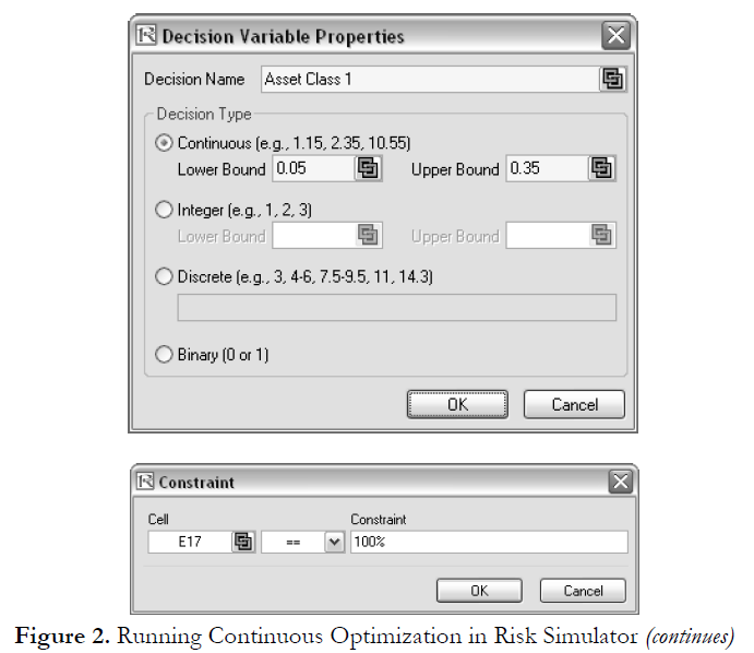
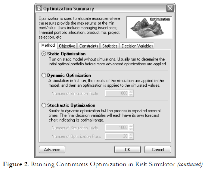
Figure 2 shows the screen shots of the preceding procedural steps. You can add simulation assumptions on the model’s returns and risk (columns C and D) and apply the dynamic optimization and stochastic optimization for additional practice.

Results Interpretation
The optimization’s final results are shown in Figure 3, where the optimal allocation of assets for the portfolio is seen in cells E6:E15. Given the restrictions of each asset fluctuating between 5% and 35%, and where the sum of the allocation must equal 100%, the allocation that maximizes the return to risk ratio is seen in Figure 3.

A few important things must be noted when reviewing the results and optimization procedures performed thus far:

• The correct way to run the optimization is to maximize the bang for the buck or returns to risk Sharpe Ratio as we have done.
• If instead we maximized the total portfolio returns, the optimal allocation result is trivial and does not require optimization to obtain. That is, simply allocate 5% (the minimum allowed) to the lowest 8 assets, 35% (the maximum allowed) to the highest returning asset, and the remaining (25%) to the second-best returns asset. Optimization is not required. However, when allocating the portfolio this way, the risk is a lot higher as compared to when maximizing the returns to risk ratio, although the portfolio returns by themselves are higher.
• In contrast, one can minimize the total portfolio risk, but the returns will now be less.

Table 1 illustrates the results from the three different objectives being optimized.

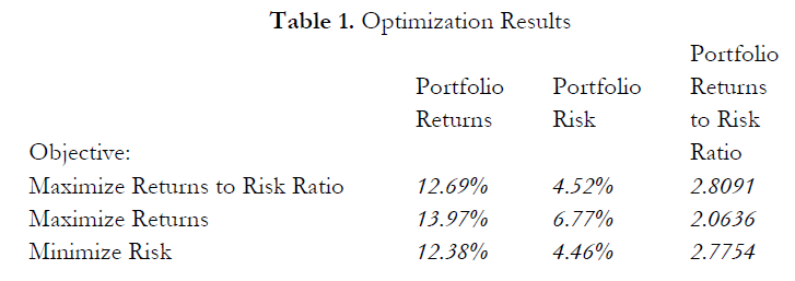
From the table, it can be seen that the best approach is to maximize the returns to risk ratio; that is, for the same amount of risk, this allocation provides the highest amount of return. Conversely, for the same amount of return, this allocation provides the lowest amount of risk possible. This approach of bang for the buck or returns to risk ratio is the cornerstone of the Markowitz efficient frontier in modern portfolio theory. That is, if we constrained the total portfolio risk level and successively increased it, over time we would obtain several efficient portfolio allocations for different risk characteristics. Thus, different efficient portfolio allocations can be obtained for different individuals with different risk preferences.