Optimization Procedures: Discrete Binary Optimization

• By Admin
• September 17, 2014
• Comments Off on Optimization Procedures: Discrete Binary Optimization

Many algorithms exist to run optimization and many different procedures exist when optimization is coupled with Monte Carlo simulation. In Risk Simulator, there are three distinct optimization procedures and optimization types as well as different decision variable types. For instance, Risk Simulator can handle Continuous Decision Variables (1.2535, 0.2215, and so forth), Integer Decision Variables (e.g., 1, 2, 3, 4 or 1.5, 2.5, 3.5, and so forth), Binary Decision Variables (1 and 0 for go and no-go decisions), and Mixed Decision Variables (both integers and continuous variables). On top of that, Risk Simulator can handle Linear Optimization (i.e., when both the objective and constraints are all linear equations and functions) and Nonlinear Optimizations (i.e., when the objective and constraints are a mixture of linear and nonlinear functions and equations).

As far as the optimization process is concerned, Risk Simulator can be used to run a Discrete Optimization, that is, an optimization that is run on a discrete or static model, where no simulations are run. In other words, all the inputs in the model are static and unchanging. This optimization type is applicable when the model is assumed to be known and no uncertainties exist. Also, a discrete optimization can first be run to determine the optimal portfolio and its corresponding optimal allocation of decision variables before more advanced optimization procedures are applied. For instance, before running a stochastic optimization problem, a discrete optimization is first run to determine if solutions to the optimization problem exist before a more protracted analysis is performed.

Next, Dynamic Optimization is applied when Monte Carlo simulation is used together with optimization. Another name for such a procedure is Simulation-Optimization. That is, a simulation is first run, then the results of the simulation are applied in the Excel model, and then an optimization is applied to the simulated values. In other words, a simulation is run for N trials, and then an optimization process is run for M iterations until the optimal results are obtained or an infeasible set is found. Using Risk Simulator’s optimization module, you can choose which forecast and assumption statistics to use and replace in the model after the simulation is run. Then, these forecast statistics can be applied in the optimization process. This approach is useful when you have a large model with many interacting assumptions and forecasts, and when some of the forecast statistics are required in the optimization. For example, if the standard deviation of an assumption or forecast is required in the optimization model (e.g., computing the Sharpe Ratio in asset allocation and optimization problems where we have mean divided by standard deviation of the portfolio), then this approach should be used.

The Stochastic Optimization process, in contrast, is similar to the dynamic optimization procedure except that the entire dynamic optimization process is repeated T times. That is, a simulation with N trials is run, and then an optimization is run with M iterations to obtain the optimal results. Then the process is replicated T times. The results will be a forecast chart of each decision variable with T values. In other words, a simulation is run and the forecast or assumption statistics are used in the optimization model to find the optimal allocation of decision variables. Then, another simulation is run, generating different forecast statistics, and these new updated values are then optimized, and so forth. Hence, the final decision variables will each have their own forecast chart, indicating the range of the optimal decision variables. For instance, instead of obtaining single-point estimates in the dynamic optimization procedure, you can now obtain a distribution of the decision variables and, hence, a range of optimal values for each decision variable, also known as a stochastic optimization.

Finally, an Efficient Frontier optimization procedure applies the concepts of marginal increments and shadow pricing in optimization. That is, what would happen to the results of the optimization if one of the constraints were relaxed slightly? Say, for instance, that the budget constraint is set at $1 million. What would happen to the portfolio’s outcome and optimal decisions if the constraint were now $1.5 million, or $2 million, and so forth. This is the concept of the Markowitz efficient frontier in investment finance, where if the standard deviation of the portfolio is allowed to increase slightly, we want to know what additional returns the portfolio will generate. This process is similar to the dynamic optimization process with the exception that one of the constraints is allowed to change, and with each change, the simulation and optimization process is run. This process is best applied manually using Risk Simulator. This process can be run either manually (re-running the optimization several times) or automatically (using Risk Simulator’s changing constraint and efficient frontier functionality). As example, the manual process is: Run a dynamic or stochastic optimization, then rerun another optimization with a new constraint, and repeat that procedure several times. This manual process is important, as by changing the constraint, the analyst can determine if the results are similar or different, and hence, whether it is worthy of any additional analysis, or to determine how far a marginal increase in the constraint should be to obtain a significant change in the objective and decision variables. This is done by comparing the forecast distribution of each decision variable after running a stochastic optimization. Alternatively, the automated efficient frontier approach will be shown later.

One item is worthy of consideration. Other software products exist that supposedly perform stochastic optimization,
but, in fact, they do not. For instance, after a simulation is run, then one iteration of the optimization process is generated, and then another simulation is run, then the second optimization iteration is generated and so forth. This process is simply a waste of time and resources; that is, in optimization, the model is put through a rigorous set of algorithms, where multiple iterations (ranging from several to thousands of iterations) are required to obtain the optimal results. Hence, generating one iteration at a time is a waste of time and resources. The same portfolio can be solved in under a minute using Risk Simulator as compared to multiple hours using such a backward approach. Also, such a simulation-optimization approach will typically yield bad results and is not a stochastic optimization approach. Be extremely careful of such methodologies when applying optimization to your models.

The following are example optimization problems. One uses continuous decision variables while the other uses discrete integer decision variables. In either model, you can apply discrete optimization, dynamic optimization, or stochastic optimization, or even manually generate efficient frontiers with shadow pricing. Any of these approaches can be used for these examples. Therefore, for simplicity, only the model setup is illustrated and it is up to the user to decide which optimization process to run. Also, the continuous decision variable example uses the nonlinear optimization approach (because the portfolio risk computed is a nonlinear function, and the objective is a nonlinear function of portfolio returns divided by portfolio risks) while the second example of an integer optimization is an example of a linear optimization model (its objective and all of its constraints are linear). Therefore, these examples encapsulate all of the procedures aforementioned.

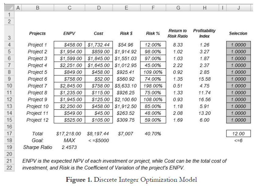
Sometimes, the decision variables are not continuous but discrete integers (e.g., 1, 2, 3) or binary (e.g., 0 and 1). We can use such binary decision variables as on-off switches or go/no-go decisions. Figure 1 illustrates a project selection model where there are 12 projects listed. The example here uses the Optimization Discrete file found on Risk Simulator | Example Models. Each project has its own returns (ENPV and NPV for expanded net present value and net present value––the is simply the NPV plus any strategic real options values), costs of implementation, risks, and so forth. If required, this model can be modified to include required full-time equivalences (FTE) and other resources of various functions, and additional constraints can be set on these additional resources. The inputs into this model are typically linked from other spreadsheet models. For instance, each project will have its own discounted cash flow or returns on investment model. The application here is to maximize the portfolio’s Sharpe Ratio subject to some budget allocation. Many other versions of this model can be created, for instance, maximizing the portfolio returns, or minimizing the risks, or adding more constraints
where the total number of projects chosen cannot exceed 6, and so forth and so on. All of these items can be run using this existing model.

Procedure

• Open the example file (Discrete Optimization) and start a new profile by clicking on Risk Simulator | New Profile and provide it a name.
• The first step in optimization is to set up the decision variables. Set the first decision variable by selecting cell J4, and select Risk Simulator | Optimization | Set Decision, click on the link icon to select the name cell (B4), and select the Binary variable. Then, using Risk Simulator copy, copy this J4 decision variable cell and paste the decision variable to the remaining cells in J5 to J15.

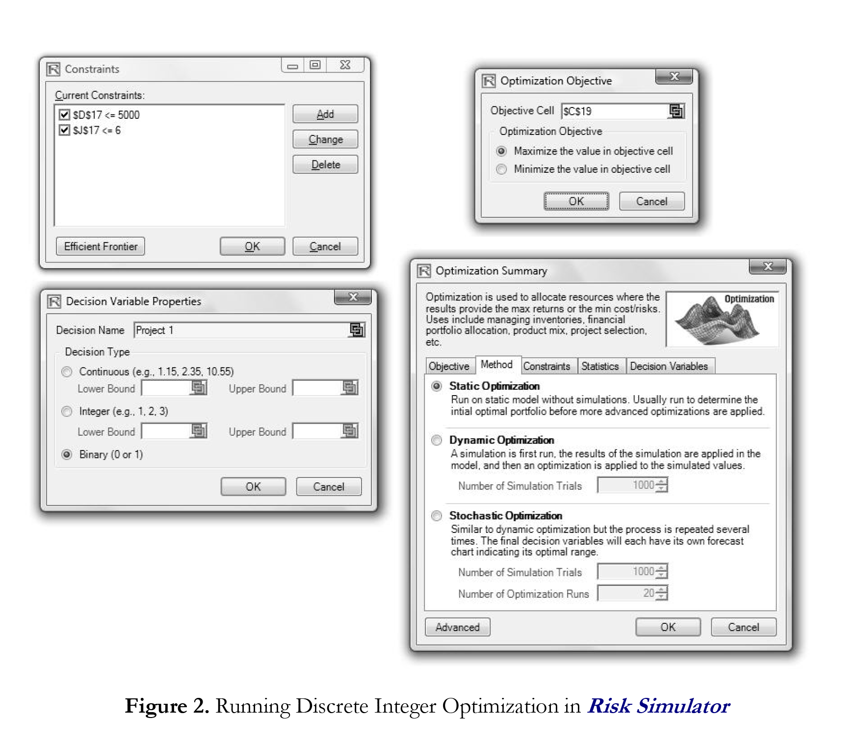
• The second step in optimization is to set the constraint. There are two constraints here, that is, the total budget allocation in the portfolio must be less than $5,000 and the total number of projects must not exceed 6. So, click on Risk Simulator | Optimization | Constraints… and select ADD to add a new constraint. Then, select the cell D17 and make it less than or equal (<=) to 5000. Repeat by setting cell J17 <= 6.
• The final step in optimization is to set the objective function and start the optimization by selecting cell C19 and selecting Risk Simulator | Optimization | Set Objective and then run the optimization (Risk Simulator | Optimization | Run Optimization) and choosing the optimization of choice (Static Optimization, Dynamic Optimization, or Stochastic Optimization). To get started, select Static Optimization. Check to make sure that the objective cell is C19 and select Maximize. You can now review the decision variables and constraints if required, or click OK to run the static optimization.

Figure 2 shows the screen shots of the foregoing procedural steps. You can add simulation assumptions on the model’s ENPV and Risk (columns C and F) and apply the dynamic optimization and stochastic optimization for additional practice.

Results Interpretation

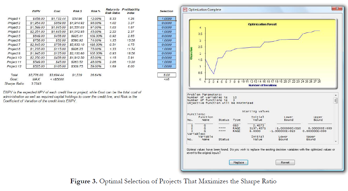
Figure 3 shows a sample optimal selection of projects that maximizes the Sharpe Ratio. In contrast, one can always maximize total revenues, but this process is trivial and simply involves choosing the highest returning project and going down the list until you run out of money or exceed the budget constraint. Doing so will yield theoretically undesirable projects as the highest yielding projects typically hold higher risks. Now, if desired, you can replicate the optimization using a stochastic or dynamic optimization by adding assumptions in the ENPV and Risk values.