Optimization Procedures: Stochastic Optimization

• By Admin
• September 17, 2014
• Comments Off on Optimization Procedures: Stochastic Optimization

Many algorithms exist to run optimization and many different procedures exist when optimization is coupled with Monte Carlo simulation. In Risk Simulator, there are three distinct optimization procedures and optimization types as well as different decision variable types. For instance, Risk Simulator can handle Continuous Decision Variables (1.2535, 0.2215, and so forth), Integer Decision Variables (e.g., 1, 2, 3, 4 or 1.5, 2.5, 3.5, and so forth), Binary Decision Variables (1 and 0 for go and no-go decisions), and Mixed Decision Variables (both integers and continuous variables). On top of that, Risk Simulator can handle Linear Optimization (i.e., when both the objective and constraints are all linear equations and functions) and Nonlinear Optimizations (i.e., when the objective and constraints are a mixture of linear and nonlinear functions and equations).

As far as the optimization process is concerned, Risk Simulator can be used to run a Discrete Optimization, that is, an optimization that is run on a discrete or static model, where no simulations are run. In other words, all the inputs in the model are static and unchanging. This optimization type is applicable when the model is assumed to be known and no uncertainties exist. Also, a discrete optimization can first be run to determine the optimal portfolio and its corresponding optimal allocation of decision variables before more advanced optimization procedures are applied. For instance, before running a stochastic optimization problem, a discrete optimization is first run to determine if solutions to the optimization problem exist before a more protracted analysis is performed.

Next, Dynamic Optimization is applied when Monte Carlo simulation is used together with optimization. Another name for such a procedure is Simulation-Optimization. That is, a simulation is first run, then the results of the simulation are applied in the Excel model, and then an optimization is applied to the simulated values. In other words, a simulation is run for N trials, and then an optimization process is run for M iterations until the optimal results are obtained or an infeasible set is found. Using Risk Simulator’s optimization module, you can choose which forecast and assumption statistics to use and replace in the model after the simulation is run. Then, these forecast statistics can be applied in the optimization process. This approach is useful when you have a large model with many interacting assumptions and forecasts, and when some of the forecast statistics are required in the optimization. For example, if the standard deviation of an assumption or forecast is required in the optimization model (e.g., computing the Sharpe Ratio in asset allocation and optimization problems where we have mean divided by standard deviation of the portfolio), then this approach should be used.

The Stochastic Optimization process, in contrast, is similar to the dynamic optimization procedure with the exception that the entire dynamic optimization process is repeated T times. That is, a simulation with N trials is run, and then an optimization is run with M iterations to obtain the optimal results. Then the process is replicated T times. The results will be a forecast chart of each decision variable with T values. In other words, a simulation is run and the forecast or assumption statistics are used in the optimization model to find the optimal allocation of decision variables. Then, another simulation is run, generating different forecast statistics, and these new updated values are then optimized, and so forth. Hence, the final decision variables will each have their own forecast chart, indicating the range of the optimal decision variables. For instance, instead of obtaining single-point estimates in the dynamic optimization procedure, you can now obtain a distribution of the decision variables and hence, a range of optimal values for each decision variable, also known as a stochastic optimization.

Finally, an Efficient Frontier optimization procedure applies the concepts of marginal increments and shadow pricing in optimization. That is, what would happen to the results of the optimization if one of the constraints were relaxed slightly? Say for instance, the budget constraint is set at $1 million. What would happen to the portfolio’s outcome and the optimal decisions if the constraint were now $1.5 million, or $2 million, and so forth. This is the concept of the Markowitz efficient frontier in investment finance, where if the portfolio standard deviation is allowed to increase slightly, we want to know what additional returns the portfolio will generate. This process is similar to the dynamic optimization process with the exception that one of the constraints is allowed to change, and with each change, the simulation and optimization process is run. This process is best applied manually using Risk Simulator. This process can be run either manually (re-running the optimization several times) or automatically (using Risk Simulator’s changing constraint and efficient frontier functionality). As example, the manual process is: Run a dynamic or stochastic optimization, then rerun another optimization with a new constraint, and repeat that procedure several times. This manual process is important, as by changing the constraint, the analyst can determine if the results are similar or different, and hence, whether it is worthy of any additional analysis, or to determine how far a marginal increase in the constraint should be to obtain a significant change in the objective and decision variables. This is done by comparing the forecast distribution of each decision variable after running a stochastic optimization. Alternatively, the automated efficient frontier approach will be shown later.

One item is worthy of consideration. Other software products exist that supposedly perform stochastic optimization, but, in fact, they do not. For instance, after a simulation is run, then one iteration of the optimization process is generated, and then another simulation is run, then the second optimization iteration is generated and so forth. This process is simply a waste of time and resources; that is, in optimization, the model is put through a rigorous set of algorithms, where multiple iterations (ranging from several to thousands of iterations) are required to obtain the optimal results. Hence, generating one iteration at a time is a waste of time and resources. The same portfolio can be solved in under a minute using Risk Simulator as compared to multiple hours using such a backward approach. Also, such a simulation-optimization approach will typically yield bad results and is not a stochastic optimization approach. Be extremely careful of such methodologies when applying optimization to your models.

The following are example optimization problems. One uses continuous decision variables while the other uses discrete integer decision variables. In either model, you can apply discrete optimization, dynamic optimization, or stochastic optimization, or even manually generate efficient frontiers with shadow pricing. Any of these approaches can be used for these examples. Therefore, for simplicity, only the model setup is illustrated and it is up to the user to decide which optimization process to run. Also, the continuous decision variable example uses the nonlinear optimization approach (because the portfolio risk computed is a nonlinear function, and the objective is a nonlinear function of portfolio returns divided by portfolio risks) while the second example of an integer optimization is an example of a linear optimization model (its objective and all of its constraints are linear). Therefore, these examples encapsulate all of the procedures aforementioned.

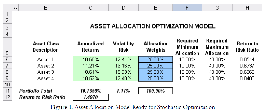
This example illustrates the application of stochastic optimization using a sample model with four asset classes each with different risk and return characteristics. The idea here is to find the best portfolio allocation such that the portfolio’s bang for the buck, or returns to risk ratio, is maximized. That is, the goal is to allocate 100% of an individual’s investment among several different asset classes (e.g., different types of mutual funds or investment styles: growth, value, aggressive growth, income, global, index, contrarian, momentum, etc.). This model is different from others because there exist several simulation assumptions (risk and return values for each asset in columns C and D), as seen in Figure 1.

A simulation is run, then optimization is executed, and the entire process is repeated multiple times to o btain distributions of each decision variable. The entire analysis can be automated using Stochastic Optimization. In order to run an optimization, several key specifications on the model have to be identified first:

The model shows the various asset classes. Each asset class has its own set of annualized returns and annualized volatilities. These return and risk measures are annualized values such that they can be consistently compared across different asset classes. Returns are computed using the geometric average of the relative returns, while the risks are computed using the logarithmic relative stock returns approach.

Column E, the Allocation Weights, holds the decision variables, which are the variables that need to be tweaked and tested such that the total weight is constrained at 100% (cell E11). Typically, to start the optimization, we will set these cells to a uniform value. In this case, cells E6 to E9 are set at 25% each. In addition, each decision variable may have specific restrictions in its allowed range. In this example, the lower and upper allocations allowed are 10% and 40%, as seen in columns F and G. This setting means that each asset class may have its own allocation boundaries.

Next, column H shows the return to risk ratio, which is simply the return percentage divided by the risk percentage for each asset, where the higher this value, the higher the bang for the buck. The remaining parts of the model show the individual asset class rankings by returns, risk, return to risk ratio, and allocation. In other words, these rankings show at a glance which asset class has the lowest risk, or the highest return, and so forth.

Running an Optimization
To run this model, simply click on Risk Simulator | Optimization | Run Optimization. Alternatively, and for practice, you can set up the model using the following steps:

1. Start a new profile (Risk Simulator | New Profile).
2. For stochastic optimization, set distributional assumptions on the risk and returns for each asset class. That is, select cell C6, set an assumption (Risk Simulator | Set Input Assumption), and make your own assumption as required. Repeat for cells C7 to D9.
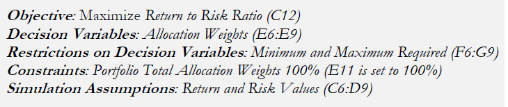
3. Select cell E6, define the decision variable (Risk Simulator | Optimization | Set Decision or click on the Set Decision D icon), and make it a Continuous Variable. Then link the decision variable’s name and minimum/maximum required to the relevant cells (B6, F6, G6).
4. Then use the Risk Simulator copy on cell E6, select cells E7 to E9, and use Risk Simulator paste (Risk Simulator | Copy Parameter and Risk Simulator | Paste Parameter, or use the copy and paste icons). Remember not to use Excel’s regular copy and paste functions.
5. Next, set up the optimization’s constraints by selecting Risk Simulator | Optimization | Constraints, selecting ADD, and selecting the cell E11 and making it equal 100% (total allocation, and do not forget the % sign).
6. Select cell C12, the objective to be maximized, and make it the objective: Risk Simulator | Optimization | Set Objective or click on the O icon.
7. Run the optimization by going to Risk Simulator | Optimization | Run Optimization. Review the different tabs to make sure that all the required inputs in steps 2 and 3 are correct. Select Stochastic Optimization and let it run for 500 trials repeated 20 times (Figure 2 illustrates these setup steps).

Click OK when the simulation completes and a detailed stochastic optimization report will be generated along with forecast charts of the decision variables.

Viewing and Interpreting Forecast Results
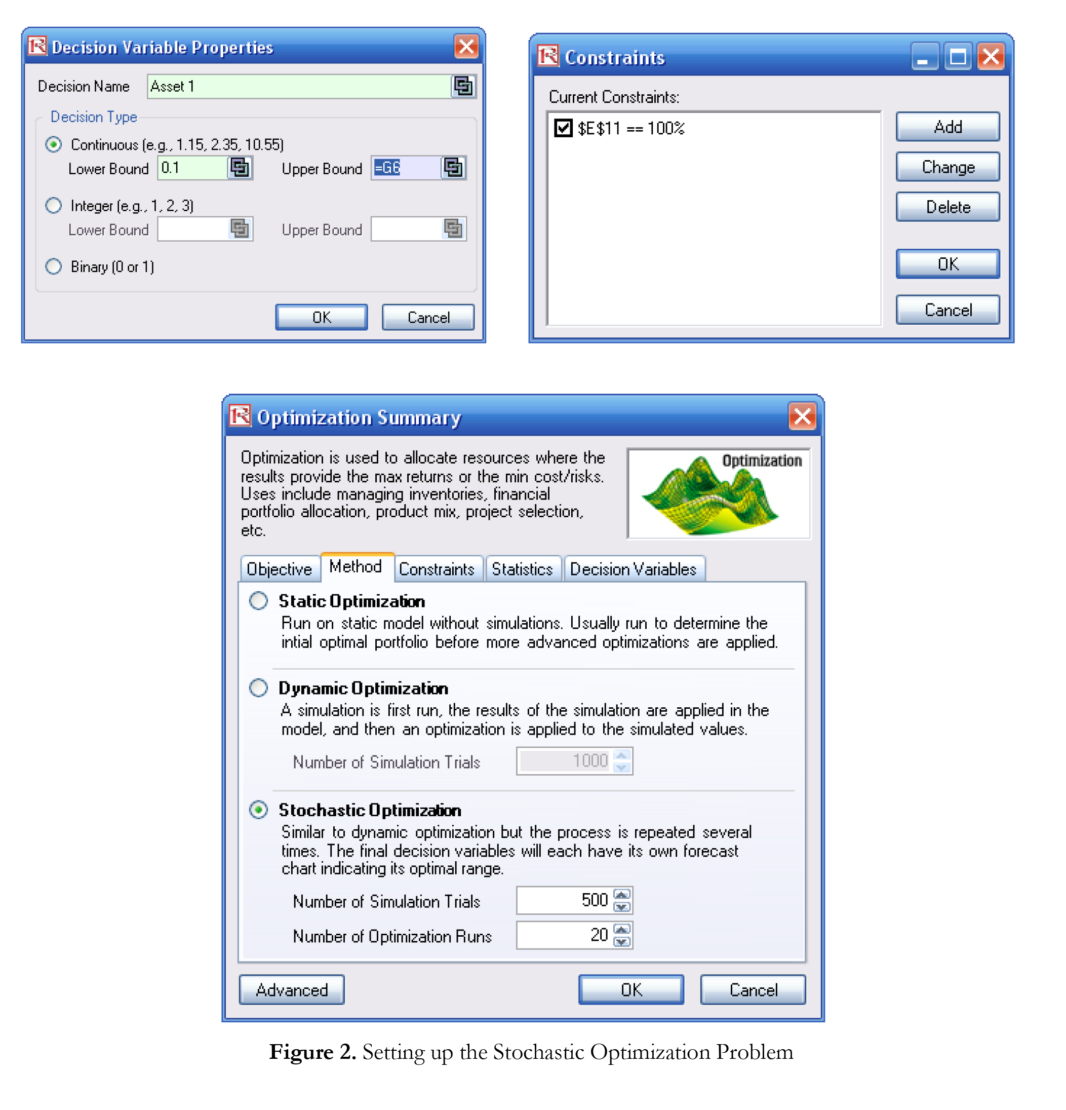
Stochastic optimization is performed when a simulation is first run and then the optimization is run. Then the whole analysis is repeated multiple times. The result is a distribution of each decision variable rather than a single-point estimate (Figure 3). So instead of saying you should invest 30.53% in Asset 1, the optimal decision is to invest between 30.19% and 30.88% as long as the total portfolio sums to 100%. This way, the results provide management or decision makers a range of flexibility in the optimal decisions, and all the while accounting for the risks and uncertainties in the inputs.

Notes

• Super Speed Simulation with Optimization. You can also run stochastic optimization with super speed simulation. To do this, first reset the optimization by resetting all four decision variables back to 25%. Next select Run Optimization, click on the Advanced button (Figure 2), and select the checkbox for Run Super Speed Simulation. Then, in the run optimization user interface, select Stochastic Optimization on the Method tab and set it to run 500 trials and 20 optimization runs, and click OK. This approach will integrate the super speed simulation with optimization. Notice how much faster the stochastic optimization runs. You can now quickly rerun the optimization with a higher number of simulation trials.
• Simulation Statistics for Stochastic and Dynamic Optimization. Notice that if there are input simulation assumptions in the optimization model (i.e., these input assumptions are required to run the dynamic or stochastic optimization routines), the Statistics tab is now populated in the Run Optimization user interface. You can select from the drop-down list the statistics you want, such as average, standard deviation, coefficient of variation, conditional mean, conditional variance, a specific percentile, and so forth. Thus, if you run a stochastic optimization, a simulation of thousands of trials will first run; then the selected statistic will be computed and this value will be temporarily placed in the simulation assumption cell; then an optimization will be run based on this statistic; then the entire process is repeated multiple times. This method is important and useful for banking applications in computing Conditional Value at Risk or Conditional VaR.