Performing Due Diligence, Part 2

• By Admin
• December 3, 2014
• Comments Off on Performing Due Diligence, Part 2

Reading the Warning Signs in Monte Carlo Simulation
Monte Carlo simulation is a very potent methodology solving difficult and often intractable problems with simplicity and ease. It creates artificial futures by generating thousands and even millions of sample paths of outcomes and looks at their prevalent characteristics. For analysts in a company, taking graduate-level advanced mathematics courses is neither logical nor practical. A brilliant analyst would use all available tools at his or her disposal to obtain the same answer the easiest way possible. One such tool is Monte Carlo simulation using
Risk Simulator. The major benefit that Risk Simulator brings is its simplicity of use. Here are seven of fourteen due-diligence issues management should evaluate when an analyst presents a report with a series of advanced analytics using simulation. The remaining seven issues are covered in “Performing Due Diligence, Part 3.”

1. How Are the Distributions Obtained?
One thing is certain: If an analyst provides a report showing all the fancy analyses undertaken and one of these analyses is the application of Monte Carlo simulation of a few dozen variables, where each variable has the same distribution (e.g., triangular distribution), management should be very worried indeed and with good reason. One might be able to accept that a few variables are triangularly distributed, but to assume that this holds true for
several dozen other variables is ludicrous. One way to test the validity of distributional assumptions is to apply historical data to the distribution and see how far off one is. Another approach is to test the alternate parameters of the distribution. For instance, if a normal distribution is used on simulating market share, and the mean is set at 55% with a standard deviation of 45%, one should be very worried. Using Risk Simulator’s alternate parameter function, the 10th and 90th percentiles indicate a value of –2.67% and 112.67%. Clearly these values cannot exist under actual conditions. How can a product have –2.67% or 112.67% of the market share? The alternate-parameters function is a very powerful tool to use in conditions such as these. Almost always, the first thing that should be done is the use of alternate parameters to ascertain the logical upper and lower values of an input parameter.

2. How Sensitive Are the Distributional Assumptions?
Obviously, not all variables under the sun should be simulated. For instance, a U.S.-based firm doing business within the 48 contiguous states should not have to worry about what happens to the foreign exchange market of the Zambian kwacha. Risk is something one bears and is the outcome of uncertainty. Just because there is uncertainty, there could very well be no risk. If the only thing that bothers a U.S.-based firm’s CEO is the fluctuation of the
Zambian kwacha, then I might suggest shorting some kwachas and shifting his or her portfolio to U.S.-based bonds.
In short, simulate when in doubt, but simulate the variables that actually have an impact on what you are trying to estimate. Make sure the simulated variables are the critical success drivers––variables that have a significant impact on the bottom line being estimated while at the same time being highly uncertain and beyond the control of management.

3. What Are the Critical Success Drivers?
Critical success drivers are related to how sensitive the resulting bottom line is to the input variables and assumptions. Before using Monte Carlo simulation, tornado charts should first be applied to help identify which variables are the most critical to analyze. Coupled with management’s and the analyst’s expertise, the relevant critical success drivers––the variables that drive the bottom line the most while being highly uncertain and beyond the control of management––can be determined and simulated. Obviously the most sensitive variables should receive the most amount of attention.

4. Are the Assumptions Related, and Have Their Relationships Been Considered?
Simply defining assumptions on variables that have significant impact without regard to their interrelationships is also a major error most analysts make. For instance, when an analyst simulates revenues, he or she could conceivably break the revenue figures into price and quantity, where the resulting revenue figure is simply the product of price and quantity. The problem is that a major error arises if both price and quantity are considered as independent variables occurring in isolation. Clearly, for most products, the law of demand in economics takes over, where the higher the price of a product, ceteris paribus, or holding everything else constant, the quantity demanded of the same product decreases. Ignoring this simple economic truth, where both price and quantity are assumed to occur independently of one another, means that the possibility of a high price and a high quantity demanded may occur simultaneously, or vice versa. Clearly this condition will never occur in real life, thus, the simulation results will most certainly be flawed. The revenue or price estimates can also be further disaggregated into several product categories, where each category is correlated to the rest of the group (competitive products, product life cycle, product substitutes, complements, and cannibalization). Other examples include the possibility of economies of scale (where a higher production level forces cost to decrease over time), product life cycles (sales tend to decrease over time and plateau at a saturation rate), average total costs (the average of fully allocated cost decreases initially and increases after it hits some levels of diminishing returns). Therefore, relationships, correlations, and causalities have to be modeled appropriately. If data are available, a simple correlation matrix can be generated through Excel to capture these relationships.

5. Have You Considered Truncation?
Truncation is a major error Risk Simulator users commit, especially when using the infamous triangular distribution. The triangular distribution is very simple and intuitive. As a matter of fact, it is probably the most widely used distribution in Risk Simulator, apart from the normal and uniform distributions. Simplistically, the triangular distribution looks at the minimum value, the most probable value, and the maximum value. These three inputs are often confused with the worstcase, nominal-case, and best-case scenarios. This assumption is indeed incorrect. In fact, a worst-case scenario can be translated as a highly unlikely condition that will still occur given a percentage of the time. For instance, one can model the economy as high, average, and low, analogous to the worst-case, nominal-case, and best-case scenarios. Thus, logic would dictate that the worst-case scenario might have, say, a 15% chance of occurrence, the nominal-case, a 50% chance of occurrence, and a 35% chance that a best-case scenario will occur. This approach is what is meant by using a best-, nominal-, and worst-case scenario analysis. However, compare that to the triangular distribution, where the minimum and maximum cases will almost never occur, with a probability of occurrence set at zero!

For instance, see Figure 1, where the worst-, nominal-, and best-case scenarios are set as 5, 10, and 15, respectively. Note that at the extreme values, the probability of 5 or 15 occurring is virtually zero, as the areas under the curve (the measure of probability) of these extreme points are zero. In other words, 5 and 15 will almost never occur. Compare that to the economic scenario where these extreme values have either a 15% or 35% chance of occurrence.

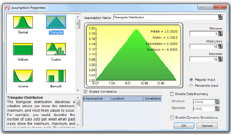Figure 1. Sample Triangular Distribution The triangular distribution describes a situation where you know the minimum, maximum, and most likely values to occur. For example, you could describe the number of cars sold per week when past sales show the minimum, maximum, and usual number of cars sold. The minimum number of items is fixed, the maximum number of items is fixed, and the most likely number of items falls between the minimum and maximum values, forming a triangular-shaped distribution, which shows that values near the minimum and maximum are less likely to occur than those near the most-likely value. Minimum value (Min), most likely value (Likely) and maximum value (Max) are the distributional
parameters.

Instead, distributional truncation should be considered here. The same applies to any other distribution. Figure 2 illustrates a truncated normal distribution where the extreme values do not extend to both positive and negative infinities, but are truncated at 7 and 13.

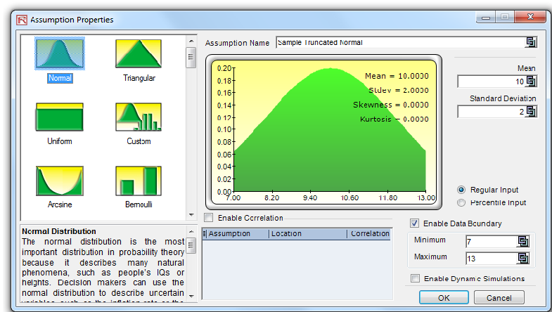
Figure 2. Truncating a Distribution Distributional truncation or data boundaries are typically not used by the average analyst but exist for truncating the distributional assumptions. For instance, if a normal distribution is selected, the theoretical boundaries are between negative infinity and positive infinity. However, in practice, the
simulated variable exists only within some smaller range, and this range can then be entered to truncate the distribution appropriately.

6. How Wide Are the Forecast Results?
I have seen models that are as large as 300 MB with over 1,000 distributional assumptions. When you have a model that big with so many assumptions, there is a huge problem! For one, it takes an unnecessarily long time to run in Excel, and for another, the results generated are totally bogus. One thing is certain: The final forecast distribution of the results will most surely be too large to make any definitive decision with. Besides, what is the use of generating results that are close to a range between negative and positive infinity?

The results that you obtain should fall within decent parameters and intervals. One good check is to simply look at the single-point estimates. In theory, the single-point estimate is based on all precedent variables at their respective expected values. Thus, if one perturbs these expected values by instituting distributions about their single-point estimates, then the resulting single-point bottom-line estimate should also fall within this forecast interval.

7. What Are the Endpoints and Extreme Values?
Mistaking end points is both an interpretation and a user error. For instance, Figure 3 illustrates the results obtained from a financial analysis with extreme values between $5.49 million and $15.49 million. By making the leap that the worst possible outcome is $5.49 million and the best possible outcome is $15.49 million, the analyst has made a major error.

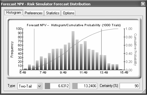
Figure 3. Truncated Extreme Values

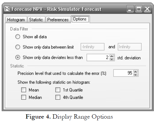
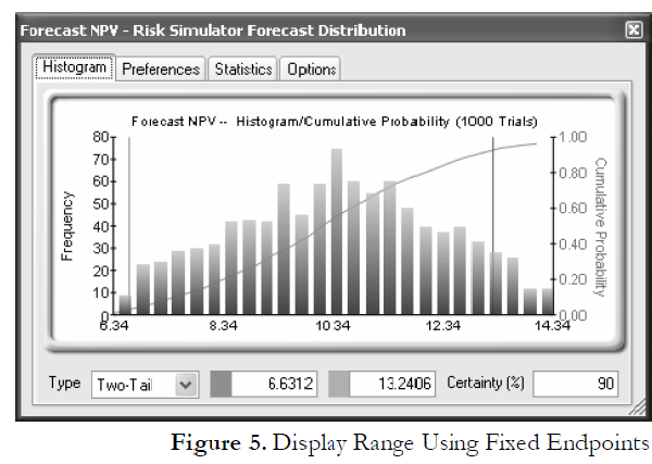
Clicking on the Options menu and selecting Display Range, one can choose any display range (Figure 4). Clearly, if the show data less than 2 standard deviation option is chosen, the graph looks somewhat different (the endpoints are now 6.34 and 14.34 as compared to 5.49 and 15.49), indicating the actual worst and best cases (Figure 5). Of course, the interpretation would be quite different here than with the 2 standard deviations option chosen.

TO BE CONTINUED IN “Performing Due Diligence, Part 3”