Performing Due Diligence, Part 3

• By Admin
• December 5, 2014
• Comments Off on Performing Due Diligence, Part 3

Reading the Warning Signs in Monte Carlo Simulation
(continued from “Performing Due Diligence, Part 2”)

“Performing Due Diligence, Part 2” covers seven of fourteen due-diligence issues management should evaluate when an analyst presents a report with a series of advanced analytics using simulation. The remaining seven such concerns are covered in this issue.

8. Are There Breaks Given Business Logic and Business Conditions?
Assumptions used in the simulation may be based on valid historical data, which means that the distributional outcomes would be valid if the firm indeed existed in the past. However, going forward, historical data may not be the best predictor of the future. In fact, past performance is no indicator of future ability to perform, especially when structural breaks in business conditions are predicted to occur. Structural breaks include
situations where firms decide to go global, acquire other firms, divest part of their assets, enter into new markets, and so forth. The resulting distributional forecasts need to be revalidated based on these conditions. The results based on past performance could be deemed as the base-case scenario, with additional adjustments and add-ons as required. This situation is especially true in the research and development arena, where things that
are yet to be developed are new and novel in nature; thus by definition, there exist no historical data on which to base the future forecasts. In situations such as these, it is best to rely on experience and expert opinions of future outcomes. Other approaches where historical data do not exist include using market proxies and project comparables––where current or historical projects and firms with similar functions, markets, and risks are used
as benchmarks.

9. Do the Results Fall Within Expected Economic Conditions?
One of the most dangerous traps analysts fall into is the trap of data mining. Rather than relying on solid theoretical frameworks, analysts let the data sort things out by themselves. For instance, analysts who blindly use stepwise regression and distributional fitting fall directly into this data-mining trap. Instead of relying on theory a priori, or before the fact, analysts use the results to explain the way things look, a posteriori, or after the fact.

A simple example is the prediction of the stock market. Using tons of available historical data on the returns of the Standard & Poor’s 500 index, an analyst runs a multivariate stepwise regression using over a hundred different variables ranging from economic growth, gross domestic product, and inflation rates, to the fluctuations of the Zambian kwacha, to who won the Super Bowl and the frequency of sunspots on particular days. Because the stock market by itself is unpredictable and random in nature, as are sunspots, there seems to be some relationship over time. Although this relationship is purely spurious and occurred out of happenstance, a stepwise regression and correlation matrix will still pick up this spurious relationship and register the relationship as statistically significant. The resulting analysis will show that sunspots do in fact explain fluctuations in the stock market. Therefore, is the analyst correct in setting up distributional assumptions based on sunspot activity in the hopes of beating the market? When one throws a computer at data, it is almost certain that a spurious connection will emerge.

The lesson learned here is to look at particular models with care when trying to find relationships that may seem on the surface to be valid, but in fact are spurious and accidental in nature, and that holding all else constant, the relationship dissipates over time. Merely correlating two randomly occurring events and seeing a relationship is nonsense and the results should not be accepted. Instead, analysis should be based on economic and financial
rationale. In this case, the economic rationale is that the relationship between sunspots and the stock market is completely accidental and should thus be treated as such.

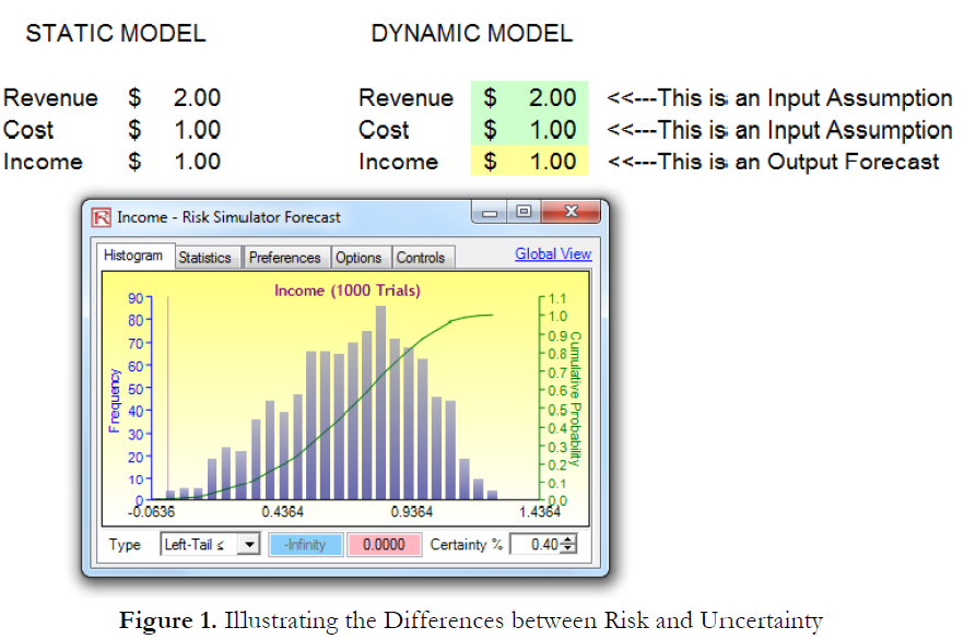
10. What Are the Values at Risk?
When applying Monte Carlo simulation, an analyst is looking at uncertainty. That is, distributions are applied todifferent variables that drive a bottom-line forecast. Figure 1 shows a very simple calculation, where on a deterministic basis, if revenue is $2 and cost is $1, the resulting net income is simply $1 (i.e., $2 – $1). However, in the dynamic model, where revenue is “around $2” and cost is “around $1,” the net income is “around $1.” This “around” comment signifies the uncertainty involved in each of these variables. The resulting variable will also be an “around” number. In fact, when Risk Simulator is applied, the resulting single-point estimate also ends up being $1. The only difference is that there is a forecast distribution surrounding this $1 value. By performing Monte Carlo simulation, a level of uncertainty surrounding this single-point estimate is obtained. Risk analysis has not yet been done. Only uncertainty analysis has been done thus far. By running simulations, only the levels of uncertainty have been quantified if the reports are shown but the results are not used to adjust for risk.

For instance, one can in theory simulate everything under the sun, including the fluctuations of the Zambian kwacha, but if the Zambian kwacha has no impact on the project being analyzed, not to mention that capturing the uncertainty surrounding the currency does not mean one has managed, reduced, or analyzed the project’s foreign exchange risks. It is only when the results are analyzed and used appropriately that risk analysis will have been done.Holding everything else constant, the best project is clearly the first project, where in the worst-case scenario 5% of the time, the minimum…

11. How Do the Assumptions Compare to Historical Data and Knowledge?
Suspect distributional assumptions should be tested through the use of backcasting, which uses historical data to test the validity of the assumptions. One approach is to take the historical data, fit them to a distribution using Risk Simulator’s distributional-fitting routines, and test the assumption inputs. See if the distributional-assumption values fall within this historical distribution. If they fall outside of the distribution’s normal set of parameters (e.g., 95% or 99% confidence intervals), then the analyst should be better able to describe and explain this apparent discontinuity, which can very well be because of changing business conditions and so forth.

12. How Do the Results Compare Against Traditional Analysis?
A very simple test of the analysis results is through its single-point estimates. For instance, remember the $1 net income example in item #10? If the single-point estimate shows $1 as the expected value of net income, then, in theory, the uncertainty surrounding this $1 should have the initial single-point estimate somewhere within its forecast distribution. If $1 is not within the resulting forecast distribution, something is amiss here. Either the model used to calculate the original $1 single-point estimate is flawed or the simulation assumptions are flawed. To recap, how can “around $2” minus “around $1” not be “around $1”?

13. Do the Statistics Confirm the Results?
Risk Simulator provides a wealth of statistics after performing a simulation. Figure 2 shows a sample listing of these statistics, which can be obtained through the View | Statistics menu in Risk Simulator. Some of these statistics when used in combination provide a solid foundation of the validity of the results. When in doubt as to what the normal looking statistics should be, simply run a simulation in Risk Simulator and set the distribution to normal with a mean of 0.00 and a standard deviation of 1.00. This condition would create a standard-normal distribution, one of the most basic statistical distributions. The resulting set of statistics is shown in Figure 2.

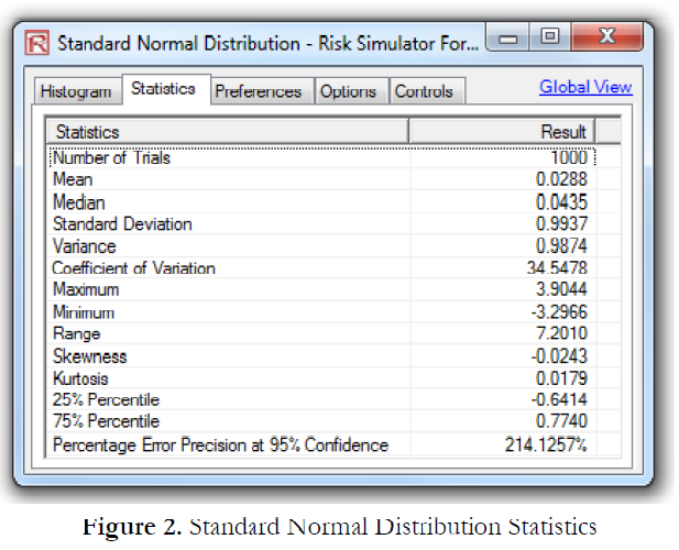
Clearly, after running 10,000 trials, the resulting mean is 0.00 with a standard deviation of 1.00, as specified in the assumption. Of particular interest are the skewness and kurtosis values. For a normally distributed result, the skewness is close to 0.00, and the excess kurtosis is close to 0.00. If the results from your analysis fall within these parameters, it is clear that the forecast values are symmetrically distributed with no excess areas in the tail. A highly positive or negative skew would indicate that something might be going on in terms of some distributional assumptions that are skewing the results either to the left or to the right. This skew may be intentional or something is amiss in terms of setting up the relevant distributions. Also, a significantly higher kurtosis value would indicate that there is a higher probability of occurrence in the tails of the distribution, which means extreme values or catastrophic events are prone to occur more frequently than predicted in most normal circumstances. This result may be expected or not. If not, then the distributional assumptions in the model should be revisited with greater care, especially the extreme values of the inputs.

14. Are the Correct Methodologies Applied?
The problem of whether the correct methodology is applied is where user error comes in. The analyst should be able
to clearly justify why a lognormal distribution is used instead of a uniform distribution and so forth, why distributional fitting is used instead of bootstrap simulation, or why a tornado chart is used instead of a sensitivity chart. All of these methodologies and approaches require some basic levels of understanding, and exploring questions such as these is most certainly required as part of management’s due diligence when evaluating an analyst’s results.

Parts 2 and 3 of “Performing Due Diligence” encompass the topic of reading the warning signs in Monte Carlo simulation by presenting fourteen due-diligence issues management should evaluate when an analyst presents a report
with a series of advanced analytics using simulation. Part 4 begins coverage of the warning signs in time-series
forecasting and regression.

TO BE CONTINUED IN “Performing Due Diligence, Part 4”