Performing Due Diligence, Part 4

• By Admin
• December 8, 2014
• Comments Off on Performing Due Diligence, Part 4

Reading the Warning Signs in Time-Series Forecasting and Regression

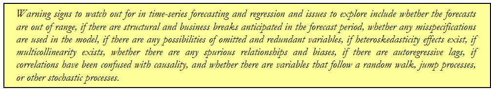
In addition to Monte Carlo simulation, another frequently used decision-analysis tool is forecasting. One thing is certain: You can never predict the future with perfect accuracy. The best that you can hope for is to get as close as possible. In addition, it is actually okay to be wrong on occasion. As a matter of fact, it is sometimes good to be wrong, as valuable lessons can be learned along the way. It is better to be wrong consistently than to be wrong on occasion because if you are wrong consistently in one direction, you can correct or reduce your expectations, or increase your expectations when you are consistently overoptimistic or underoptimistic. The problem arises when you are occasionally right and occasionally wrong, and you have no idea when or why. Here are 12 issues that should be addressed when evaluating time-series or any other forecasting results.

1. Out of Range Forecasts
Not all variables can be forecast using historical data. For instance, did you know that you can predict, rather reliably, the ambient temperature given the frequency of cricket chirps? Collect a bunch of crickets and change the ambient temperature, collect the data, and run a bivariate regression, and you will get a high level of confidence as seen in the coefficient of determination or R-squared value. Given this model, you could reasonably predict ambient temperature whenever crickets chirp, correct? Well, if you answered yes, you have just fallen
into the trap of forecasting out of range. Suppose your model holds up to statistical scrutiny, which it may very well do, assuming you do a good job with the experiment and data collection. Using the model, one finds that crickets chirp more frequently the higher the ambient temperature, and less frequently the colder if gets. What do you presume would happen if one were to toss a poor cricket in the oven and turn it up to 550 degrees? What happens when the cricket is thrown into the freezer instead? What would occur if a Malaysian cricket were used instead of the Arizona reticulated cricket? The quick answer is you can toss your fancy statistical regression model out the window if any of these things happened. As for the cricket in the oven, you would most probably hear the poor thing give out a very loud chirp and then complete silence. Regression and prediction models out of sample, that is, modeling events that are out of place and out of the range of the data collected in ordinary circumstances, on occasion will fail to work, as is clearly evident from the poor cricket.

2. Structural Breaks
Structural breaks in business conditions occur all the time. Some example instances include going public, going private, merger, acquisition, geographical expansion, adding new distribution channels, existence of new competitive threats, union strikes, change of senior management, change of company vision and long-term strategy, economic downturn, and so forth. Suppose you are an analyst at FedEx performing volume, revenue, and profitability metric forecasting of multiple break-bulk stations. These stations are located all around the United States and each station has its own seasonality factors complete with detailed historical data. Some advanced econometric models are applied, ranging from ARIMA (autoregressive integrated moving average) and ECM (error correction models) to GARCH (generalized autoregressive conditional heteroskedasticity) models; these time-series forecasting models usually provide relatively robust forecasts. However, within a single year, management reorganization, union strikes, pilot strikes, competitive threats (UPS, your main competitor…decided to enter a new submarket), revised accounting rules, and a plethora of other coincidences simply made all the forecasts invalid. The analyst must decide if these coincidences are just that, coincidences, or if they point to a fundamental structural change in the way global freight businesses are run. Obviously, certain incidences are planned or expected, whereas others are unplanned and unexpected. The planned incidences should thus be considered when performing forecasting.

3. Specification Errors
Sometimes, models are incorrectly specified. A nonlinear relationship can be very easily masked through the estimation of a linear model. Another specification error that is fairly common has to do with autocorrelated and seasonal data sets. Estimating the demand of flowers in a floral chain without accounting for the holidays (Valentine’s Day, Mother’s Day, and so forth) is a blatant specification error. Failure to clearly use the correct model specification or first sanitizing the data may result in highly erroneous results.

4. Omitted and Redundant Variables
When regression is used to forecast the future, omitted and redundant variables cause model error. Suppose an analyst uses multivariate regression to obtain a statistical relationship between a dependent variable (e.g., sales, prices, revenues) and other regressors or independent variables (e.g., economic conditions, advertising levels, market competition), and he or she hopes to use this relationship to forecast the future. Unfortunately, the analyst may not have all the available information at his or her fingertips. If important information is unavailable, an important variable may be omitted (e.g., market saturation effects, price elasticity of demand, threats of emerging technology), or if too much data is available, redundant variables may be included in the analysis (e.g., inflation rate, interest rate, economic growth). It may be counter intuitive but the problem of redundant variables is more serious than omitted variables. In a situation where redundant variables exist , and if these redundant variables are perfectly correlated or collinear with each other, the regression equation does not exist and cannot be solved. In the case where slightly less severe collinearity exists, the estimated regression equation will be less accurate than without this collinearity. For instance, suppose both interest rates and inflation rates are used as explanatory variables in the regression analysis, where if there is a significant negative correlation between these variables with a time lag, then using both variables to explain sales revenues in the future is redundant. Only one variable is sufficient to explain the relationship with sales. If the analyst uses both variables, the errors in the regression analysis will increase. The prediction errors of an additional variable will increase the errors of the entire regression.

5. Heteroskedasticity
If the variance of the errors in a regression analysis increases over time, the regression equation is said to be flawed and suffers from heteroskedasticity. Although this may seem to be a technical matter, many regression practitioners fall into this heteroskedastic trap without even realizing it.

6. Multicollinearity
One of the assumptions required for a regression to run is that the independent variables are noncorrelated or noncollinear. These independent variables are exactly collinear when a variable is an exact linear combination of the other variables. This error is most frequently encountered when dummy variables are used. A quick check of multicollinearity is to run a correlation matrix of the independent variables. In most instances, the multicollinearity problem will prevent the regression results from being computed.

7. Spurious Regression, Data Mining, Time Dependency, and Survivorship Bias
Spurious regression is another danger that analysts often run into. This mistake is made through certain uses of data-mining activities. Data mining refers to using approaches such as a step-wise regression analysis, where analysts do not have some prior knowledge of the economic effects of what independent variables drive the dependent variable, and use all available data at their disposal. The analyst then runs a step-wise regression, where the methodology ranks the highest correlated variable to the least correlated variable. Then the methodology automatically adds each successive independent variable in accordance with its correlation until some specified stopping statistical criteria. The resulting regression equation is then taken as the final and best result. The problem with this approach is that some independent variables may simply be randomly moving about while the dependent variable may also be randomly moving about, and their movements depend on time. Suppose this randomness in motion is somehow related at certain points in time but the actual economic fundamentals or financial relationships do not exist. Data-mining activities will pick up the coincidental randomness and not the actual relationship, and the result is a spurious regression. That is, the relationship estimated is bogus and is purely a chance happenstance. Multicollinearity effects may also unnecessarily eliminate highly significant variables from the stepwise regression.

Survivorship bias and self-selection bias are important considerations, as only the best-performing realization will always show up and have the most amount of visibility. For instance, looking to the market to obtain proxy data can be dangerous for only successful firms will be around and have the data. Firms that have failed will most probably leave no trails of their existence, let alone credible market data for an analyst to collect. Self-selection occurs when the data that exist are biased and selective. For instance, pharmacology research on a new cancer treatment will attract cancer patients of all types, but the researchers will clearly only select those patients in the earlier stages of cancer, making the results look more promising than they actually are.

8. Autoregressive Processes, Lags, Seasonality, and Serial Correlation
In time-series data, certain variables are autoregressive in nature. That is, future values of variables such as price, demand, interest rates, inflation rates, and so forth depend on values that occurred in the past, or are autoregressive. This reversion to the past occurs because of many reasons, including seasonality and cyclicality. Because of these cyclical or seasonal and autoregressive effects, regression analysis using seasonal or cyclical independent variables as is will yield inexact results. In fact, some of these autoregressive, cyclical, or seasonal variables will affect the dependent variable differently over time. There may be a time lag between effects; for example, an increase in interest rates may take 1 to 3 months before the mortgage market feels the effects of this decline. Ignoring this time lag will downplay the relationships of highly significant variables.

9. Correlation and Causality
Regression analysis looks at correlation effects, not causality. To say that there is a cause in X (independent variable) that drives the outcome of Y (dependent variable) through the use of regression analysis is flawed. For instance, there is a high correlation between the number of shark attacks and lunch hour around the world. Clearly, sharks cannot tell that it is time to have lunch. However, lunchtime is the warmest time of the day and is also the hour that beaches around the world are most densely populated. With a higher population of swimmers, the chances of heightened shark attacks are almost predictable. Therefore, lunchtime does not cause sharks to go hungry and prompt them to search for food. Just because there is a correlation does not mean that there is causality. Making this leap will provide analysts and management an incorrect interpretation of the results.

10. Random Walks
Certain financial data (e.g., stock prices, interest rates, inflation rates) follow something called a random walk. Random walks can take on different characteristics, including random walks with certain jumps, random walks with a drift rate, or a random walk that centers or reverts to some long-term average value. Even the models used to estimate random walks are varied, from geometric to exponential, among other things. A simple regression equation will yield no appreciable relationship when random walks exist.

11. Jump Processes
Jump processes are more difficult to grasp but are nonetheless important for management to understand to be able to challenge the assumptions of an analyst’s results. For instance, the price of oil in the global market may sometimes follow a jump process. When the United States goes to war with another country, or when OPEC decides to cut the production of oil by several billion barrels a year, oil prices will see a sudden jump. Forecasting revenues based on these oil prices overtime using historical data may not be the best approach. These sudden probabilistic jumps should most certainly be accounted for in the analysis. In this case, a jump-diffusion stochastic model is more appropriate than simple time-series or regression analyses.

12. Stochastic Processes
Other stochastic processes are also important when analyzing and forecasting the future. Interest rates and inflation rates may follow a mean-reversion stochastic process. That is, interest rates and inflation rates cannot increase or decrease so violently that they fall beyond all economic rationale. In fact, economic factors and pressures will drive these rates to their long-run averages over time. Failure to account for these effects over the long run may yield statistically incorrect estimates, resulting in erroneous forecasts.

TO BE CONCLUDED IN “Performing Due Diligence, Part 5”