QUICK OVERVIEW OF PROBABILITY DISTRIBUTIONS

• By Admin
• June 16, 2014
• Comments Off on QUICK OVERVIEW OF PROBABILITY DISTRIBUTIONS

QUICK OVERVIEW OF PROBABILITY DISTRIBUTIONS
The following is a quick synopsis of the probability distributions available in Real Options Valuation, Inc.’s various software applications such as Risk Simulator, Real Options SLS, ROV Quantitative Data Miner, ROV Modeler, and others.

PROBABILITY DISTRIBUTIONS: MOST COMMONLY USED
There are anywhere from 42 to 50 probability distributions available in the ROV software suite, and the most commonly used probability distributions are listed here in order of popularity of use. See the user manual for more technical details.

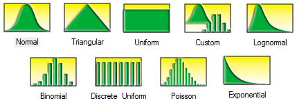
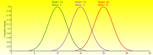
Normal. The most important distribution in probability theory, it describes many natural phenomena (people’s IQ or height, inflation rate, future price of gasoline, etc.). The uncertain variable could as likely be above the mean as below the mean (symmetrical about the mean), and the uncertain variable is more likely to be in the vicinity of the mean rather than further away. Mean (μ) <=> 0 and Standard Deviation (σ) > 0.

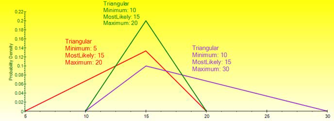
Triangular. The minimum, maximum, and most likely values are known from past data or expectations. The distribution forms a triangular shape, which shows that values near the minimum and maximum are less likely to occur than those near the most-likely value. Minimum ≤ Most Likely ≤ Maximum, but all three cannot have identical values.

Uniform. All values that fall between the minimum and maximum occur with equal likelihood and the distribution is flat. Minimum < Maximum.

Custom. The custom nonparametric simulation distribution is a data-based empirical distribution in which available historical or comparable data are used to define the custom distribution, and the simulation is distribution-free and, hence, does not require any input parameters (nonparametric). This means that
we let the data define the distribution and do not explicitly force any distribution on the data. The data is sampled with replacement repeatedly using the Central Limit Theorem.

Lognormal. Used in situations where values are positively skewed, for example, in financial analysis for security valuation or in real estate for property valuation, and where values cannot fall below zero (e.g., stock prices and real estate prices are usually positively skewed rather than Normal or symmetrically distributed and cannot fall below the lower limit of zero but might increase to any price without limit). Mean (µ) > 0 and Standard Deviation (σ) > 0.

Binomial. Describes the number of times a particular event occurs in a fixed number of trials, such as the number of heads in 10 flips of a coin or the number of defective items out of 50 items chosen. For each trial, only two mutually exclusive outcomes are possible, and the trials are independent, where
what happens in the first trial does not affect the next trial. The probability of an event occurring remains the same from trial to trial. Probability of Success 0 < (P) < 1 and the number of total Trials (N) > 0 and is a positive integer.

Discrete Uniform. Known as the equally likely outcomes distribution, where the distribution has a set of N elements, then each element has the same probability, creating a flat distribution. This distribution is related to the uniform distribution but its elements are discrete and not continuous. Minimum < Maximum, and both are integers.

Poisson. Describes the number of times an event occurs in a given interval, such as the number of telephone calls per minute or the number of errors per page in a document. The number of possible occurrences in any interval is unlimited and the occurrences are independent. The number of occurrences in
one interval does not affect the number of occurrences in other intervals, and the average number of occurrences must remain the same from interval to interval. 0 < Average Rate (λ) ≤ 1000.

Exponential. Widely used to describe events recurring at random points in time, for example, the time between events such as failures of electronic equipment or the time between arrivals at a service booth. It is related to the Poisson distribution, which describes the number of occurrences of an event in a given interval of time. An important characteristic of the exponential distribution is its memory less property, which means that the future lifetime of a given object has the same distribution regardless of the time it existed. In other words, time has no effect on future outcomes. Success Rate (λ) > 0.

PROBABILITY DISTRIBUTIONS: ALL OTHERS

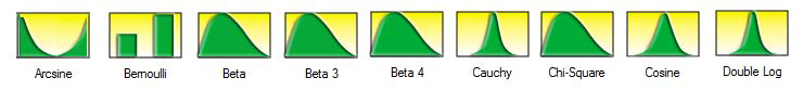
Arcsine. U-shaped, it is a special case of the Beta distribution when both shape and scale are equal to 0.5. Values close to the minimum and maximum have high probabilities of occurrence whereas values between these two extremes have very small probabilities or occurrence. Minimum < Maximum.

Bernoulli. Discrete distribution with two outcomes (e.g., head or tails, success or failure), which is why it is also known simply as the Yes/No distribution. The Bernoulli distribution is the Binomial distribution with one trial. This distribution is the fundamental building block of other more complex distributions. Probability of Success 0 < (P) < 1.

Beta. This distribution is very flexible and is commonly used to represent variability over a fixed range. It is used to describe empirical data and predict the random behavior of percentages and fractions, as the range of outcomes is typically between 0 and 1. The value of the Beta distribution lies in the wide variety of shapes it can assume when you vary the two parameters, alpha and beta. The uncertain variable is a random value between 0 and a positive value, and the shape of the distribution can be specified using two positive values. If the parameters are equal, the distribution is symmetrical. If either parameter is 1 while the other parameter is greater than 1, the distribution is triangular or J-shaped. If alpha is less than beta, the distribution is said to be positively skewed (most of the values are near the minimum value). If alpha is greater than beta, the distribution is negatively skewed (most of the values are near the maximum value). Alpha (α) > 0 and Beta (β) > 0 and can be any positive value.

Beta 3. The original Beta distribution only takes two inputs, Alpha and Beta shape parameters. However, the output of the simulated value is between 0 and 1. In the Beta 3 distribution, we add an extra parameter called Location or Shift, where we are not free to move away from this 0 to 1 output limitation, therefore the Beta 3 distribution is also known as a Shifted Beta distribution. The mathematical constructs for the Beta 3 and Beta 4 distributions are based on those in the Beta distribution, with the relevant shifts and factorial multiplication (e.g., the PDF and CDF will be adjusted by the shift and factor, and some of the moments, such as the mean, will similarly be affected; the standard deviation, in contrast, is only affected by the factorial multiplication, whereas the remaining moments are not affected at all). Alpha (α) > 0 and Beta (β) > 0 and can be any positive value; Location can take on any value.

Beta 4. Beta 4 distribution adds two input parameters to the original Beta distribution, Location, or Shift, and Factor. The original Beta distribution is multiplied by the factor and shifted by the location, and, therefore the Beta 4 is also known as the Multiplicative Shifted Beta distribution. Alpha (α) > 0 and Beta (β) > 0 and can be any positive value; Location can take on any value, and Factor > 0.

Cauchy. The Cauchy distribution, also called the Lorentzian distribution or Breit- Wigner distribution, is a continuous distribution describing resonance behavior. It also describes the distribution of horizontal distances at which a line segment tilted at a random angle cuts the x-axis. Location (α) and Scale (β) are the only two parameters in this distribution. The location parameter specifies the peak or
mode of the distribution while the scale parameter specifies the half-width at half maximum of the distribution. In addition, the mean and variance of a Cauchy or Lorentzian distribution are undefined. Location (α) can be anything and Scale (β) > 0 and can be any positive value.

Chi-Square. A distribution used predominantly in hypothesis testing, it is related to the Gamma distribution and the standard normal distribution. For instance, the sums of independent Normal distributions are distributed as a Chi-Square (X²) with k degrees of freedom. Degrees of Freedom > 1 and must be integers < 300.

Cosine. Looks like a Logistic distribution where the median value between the minimum and maximum have the highest peak or mode, carrying the maximum probability of occurrence, while the extreme tails close to the minimum and maximum values have lower probabilities. Minimum < Maximum.

Double Log. Looks like the Cauchy where the central tendency is peaked and carries the maximum value probability density but declines faster the further it gets away from the center, creating a symmetrical distribution with an extreme peak in between the minimum and maximum values. Minimum < Maximum.

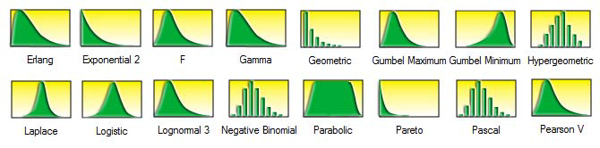
Erlang. Same as the Gamma distribution with the requirement that the Alpha or shape parameter must be a positive integer. An example application of the Erlang distribution is to calibrate the rate of transition of elements through a system of compartments. Such systems are widely used in biology and ecology (e.g., in epidemiology, an individual may progress at an exponential rate from being healthy to becoming a disease carrier, and continue exponentially from being a carrier to being infectious). Shape (α) > 0 and must be an integer, while Scale (β) > 0 can be any positive value.

Exponential 2. This distribution uses the same constructs as the original Exponential distribution but adds a Location or Shift parameter. The Exponential distribution starts from a minimum value of 0, whereas this Exponential 2, or Shifted Exponential, distribution shifts the starting location to any other value. Rate (λ) > 0 and Location can be any positive or negative value including zero.

F. The F distribution, also known as the Fisher-Snedecor distribution, is also another continuous distribution used most frequently for hypothesis testing. Specifically, it is used to test the statistical difference between two variances in analysis of variance tests and likelihood ratio tests. The Numerator Degrees of Freedom (N) > 1 and Denominator Degrees of Freedom (M) > 1 and both must be integers.

Gamma. This distribution applies to a wide range of physical quantities and is related to other distributions: Lognormal, Exponential, Pascal, Erlang, Poisson, and Chi-Square. It is used in meteorological processes to represent pollutant concentrations and precipitation quantities. The Gamma distribution is also used to measure the time between the occurrences of events when the event process is not completely random. Other applications of the Gamma distribution include inventory control, economic theory, and insurance risk theory. The number of possible occurrences in any unit of measurement is not limited to a fixed number, the occurrences are independent, the number of occurrences in one unit of measurement does not affect the number of occurrences in other units, and the average number of occurrences must remain the same from unit to unit. Shape (α) ≥ 0.5 and Scale (β) > 0. When the alpha parameter is a positive integer, the Gamma distribution is called the Erlang distribution, used to predict waiting times in queuing systems.

Geometric. A discrete distribution describing the number of trials until the first successful occurrence, such as the number of times you need to spin a roulette wheel before you win. The number of trials is not fixed, the trials continue until the first success, and the probability of success is the same from trial to trial. Probability of Success 0 < (P) < 1.

Gumbel Maximum. The extreme value distribution (Type 1) is commonly used to describe the largest value of a response over a period of time, for example, in flood flows, rainfall, and earthquakes. Other applications include the breaking strengths of materials, construction design, and aircraft loads and tolerances. The Extreme Value distribution is also known as the Gumbel distribution. The maximum extreme value distribution is positively skewed, with a higher probability of lower values and lower probability of higher extreme values. This distribution is the mirror reflection of the minimum Extreme Value distribution at the mode. Mode (α) can take on any value while Scale (β) > 0.

Gumbel Minimum. The extreme value distribution (Type 1) is commonly used to describe the largest value of a response over a period of time, for example, in flood flows, rainfall, and earthquakes. Other applications include the breaking strengths of materials, construction design, and aircraft loads and tolerances. The Extreme Value distribution is also known as the Gumbel distribution. The minimum extreme value distribution is negatively skewed, with a higher probability of higher values and lower probability of lower extreme values. This distribution is the mirror reflection of the maximum Extreme Value distribution at the mode. Mode (α) can take on any value while Scale (β) > 0.

Hypergeometric. The Hypergeometric distribution trials change the probability for each subsequent trial and are called “trials without replacement.” For example, suppose a box of manufactured parts is known to contain some defective parts. You choose a part from the box, find it is defective, and remove the part from the box. If you choose another part from the box, the probability that it is defective is somewhat lower than for the first part because you have removed a defective part. If you had replaced the defective part, the probabilities would have remained the same, and the process would have satisfied the conditions for a Binomial distribution. The total number of items or elements (the population size) is a fixed number (a finite population), the population size must be less than or equal to 1750, the sample size (the number of trials) represents a portion of the population, and the known initial probability of success in the population changes after each trial. Number of items in the population or population size (N), trials sampled or sample size (n), and number of items in the population that have the successful trait or population success (Nx) are the distributional parameters. The number of successful trials in the sample is denoted x (the x-axis of the probability distribution chart). Population Size ≥ 2 and integer, Sample Size > 0 and integer, Population Successes > 0 and integer, Population Size > Population Successes, Sample Size < Population Size, Population Size is typically less than
1750, otherwise, use the Normal distribution.

Laplace. Also sometimes called the Double Exponential distribution because it can be constructed with two exponential distributions (with an additional location parameter) spliced together back-to-back, creating an unusual peak in the middle. The probability density function of the Laplace distribution is reminiscent of the normal distribution. However, whereas the Normal distribution is expressed in terms of the squared difference from the mean, the Laplace density is expressed in terms of the absolute difference from the mean, making the Laplace distribution’s tails fatter than those of the Normal distribution. When the location parameter is set to zero, the Laplace distribution’s random variable is exponentially distributed with an inverse of the scale parameter. Location (α) can take on any positive or negative value including zero, while Scale (β) > 0.

Logistic. The Logistic distribution is commonly used to describe growth, that is, the size of a population expressed as a function of a time variable. It also can be used to describe chemical reactions and the course of growth for a population or individual. Mean (α) can take on any values, whereas Scale (β) > 0 and can only take on positive values.

Lognormal 3. The Lognormal 3 distribution uses the same constructs as the original Lognormal distribution but adds a Location, or Shift, parameter. The Lognormal distribution starts from a minimum value of 0, whereas this Lognormal 3 or Shifted Lognormal distribution shifts the starting location to any other value. Mean (μ) > 0 and Standard Deviation (σ) > 0, and Location can be any positive or negative value including zero.

Negative Binomial. The Negative Binomial distribution is useful for modeling the distribution of the number of additional trials required on top of the number of successful occurrences required (R). For instance, in order to close a total of 10 sales opportunities, how many extra sales calls would you need to make above 10 calls given some probability of success in each call? The x-axis shows the number of additional calls required or the number of failed calls. The number of trials is not fixed, the trials continue until the Rth success, and the probability of success is the same from trial to trial. Probability of Success 0 < (P) < 1 and 0 < Successes Required < 8000.

Parabolic. The Parabolic distribution is a special case of the Beta distribution when Shape = Scale = 2. Values close to the minimum and maximum have low probabilities of occurrence whereas values between these two extremes have higher probabilities of occurrence. Minimum < Maximum.

Pareto. The Pareto distribution is widely used for the investigation of distributions associated with such empirical phenomena as city population sizes, the occurrence of natural resources, the size of companies, personal incomes, stock price fluctuations, and error clustering in communication circuits. Shape (α) ≥ 0.05 and Location (β) > 0.

Pascal.The Pascal distribution is useful for modeling the distribution of the number of total trials required to obtain the number of successful occurrences required. For instance, to close a total of 10 sales opportunities, how many total sales calls would you need to make given some probability of success in each call? The x-axis shows the total number of calls required, which includes successful and failed calls. The number of trials is not fixed, the trials continue until the Rth success, and the probability of success is the same from trial to trial. Pascal distribution is related to the Negative Binomial distribution. Negative Binomial distribution computes the number of events required on top of the number of successes required given some probability (in other words, the total failures), whereas the Pascal distribution computes the total number of events required (in other words, the sum of failures and successes) to achieve the successes required given some probability. Successes Required > 0 and is an integer, while Probability of Success 0 < (P) < 1.

Pearson V. The Pearson V distribution is related to the Inverse Gamma distribution, where it is the reciprocal of the variable distributed according to the Gamma distribution. Pearson V distribution is also used to model time delays where there is almost certainty of some minimum delay and the maximum delay is unbounded (e.g., delay in arrival of emergency services and time to repair a machine). Shape (α) > 0 and Scale (β) > 0.

Pearson VI. The Pearson VI distribution is related to the Gamma distribution, where it is the rational function of two variables distributed according to two Gamma distributions. Alpha 1 (also known as shape 1), Alpha 2 (also known as shape 2), and Beta (also known as scale) are the distributional parameters. Shape 1 (α1) > 0, Shape 2 (α2) > 0, Scale (β) > 0.

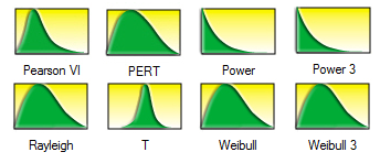
PERT. The PERT distribution is widely used in project and program management to define the worst-case, nominal-case, and best-case scenarios of project completion time. It is related to the Beta and Triangular distributions. PERT distribution can be used to identify risks in project and cost models based on the likelihood of meeting targets and goals across any number of project components using minimum, most likely, and maximum values, but it is designed to generate a distribution that more closely resembles realistic probability distributions. The PERT distribution can provide a close fit to the Normal or Lognormal distributions. Like the Triangular distribution, the PERT distribution emphasizes the “most likely” value over the minimum and maximum estimates. However, unlike the Triangular distribution, the PERT distribution constructs a smooth curve that places progressively more emphasis on values around (near) the most likely value in favor of values around the edges. In practice, this means that we “trust” the estimate for the most likely value, and we believe that even if it is not exactly accurate (as estimates seldom are), the resulting value will be close to that estimate. Assuming that many real-world phenomena are normally distributed, the appeal of the PERT distribution is that it produces a curve similar to the normal curve in shape, without knowing the precise parameters of the related normal curve. Minimum ≤ Most Likely ≤ Maximum and can be positive, negative, or zero, but all three cannot be identical.

Power. The Power distribution is related to the Exponential distribution in that the probability of small outcomes is large but exponentially decreases as the outcome value increases. Alpha (also known as shape) is the only distributional parameter. Shape (α) > 0.

Power 3. The Power 3 distribution uses the same constructs as the original Power distribution but adds a Location, or Shift, parameter, and a multiplicative Factor parameter. The Power distribution starts from a minimum value of 0, whereas this Power 3, or Shifted Multiplicative Power, distribution shifts the starting location to any other value. Shape (α) > 0.05, and Location or Shift can be any positive or negative value including zero, while Factor > 0.

Rayleigh. The Rayleigh distribution describes data resulting from life and fatigue tests. It is commonly used to describe failure time in reliability studies as well as the breaking strengths of materials in reliability and quality control tests. The Rayleigh distribution is a special case of the Weibull distribution when the shape parameter is equal to 2.0. The Weibull distribution is a family of distributions that can assume the properties of several other distributions. For example, depending on the shape parameter you define, the Weibull distribution can be used to model the exponential (when Shape = 1.0) and Rayleigh (Shape = 2.0) distributions, among others. Scale 0 < (β) ≤ 36.

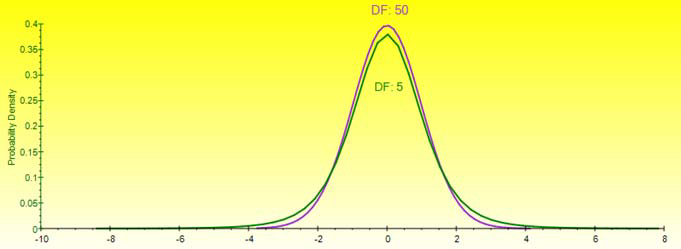
T. The Student’s T distribution is the most widely used distribution in hypothesis testing. This distribution is used to estimate the mean of a normally distributed population when the sample size is small, and is used to test the statistical significance of the difference between two sample means or confidence intervals for small sample sizes. Degrees of Freedom ≥ 1 and must be an integer.

Weibull. The Weibull distribution describes data resulting from life and fatigue tests. It is commonly used to describe failure time in reliability studies as well as the breaking strengths of materials in reliability and quality control tests. Weibull distributions are also used to represent various physical quantities, such as wind speed. The Weibull distribution is a family of distributions that can assume the properties of several other distributions. For example, depending on the shape parameter you define, the Weibull distribution can be used to model the exponential and Rayleigh distributions, among others. The Weibull distribution is very flexible. When the Weibull shape parameter is equal to 1.0, the Weibull distribution is identical to the exponential distribution. The Weibull central location scale or beta parameter lets you set up an exponential distribution to start at a location other than 0.0. When the shape parameter is less than 1.0, the Weibull distribution becomes a steeply declining curve. A manufacturer might find this effect useful in describing part failures during a burn-in period. Shape (α) ≥ 0.05 and Central Location Scale (β) > 0 and can be any positive value.

Weibull 3. The Weibull 3 distribution uses the same constructs as the original Weibull distribution but adds a Location, or Shift, parameter. The Weibull distribution starts from a minimum value of 0, whereas this Weibull 3, or Shifted Weibull, distribution shifts the starting location to any other value. Shape (α) ≥ 0.05 and Central Location Scale (β) > 0 and can be any positive value, while Location can be any positive or negative value including zero.

UNDERSTANDING PDF, CDF, AND ICDF
This section briefly explains the probability density function (PDF) for continuous distributions, which is also called the probability mass function (PMF) for discrete distributions (we use these terms interchangeably), where given some distribution and its parameters, we can determine the probability of occurrence given some outcome x. In addition, the cumulative distribution function (CDF) can also be computed, which is the sum of the PDF values up to this x value. Finally, the inverse cumulative distribution function (ICDF) is used to compute the value x given the cumulative probability of occurrence. In mathematics and Monte Carlo simulation, a probability density function (PDF) represents a continuous probability distribution in terms of integrals. If a probability distribution has a density of f(x), then intuitively the infinitesimal interval of [x, x + dx] has a probability of f(x) dx. The PDF therefore can be seen as a smoothed version of a probability histogram; that is, by providing an empirically large sample of a continuous random variable repeatedly, the histogram using very narrow ranges will resemble the random variable’s PDF. The probability of the interval between [a, b] is given by
[latexpage] \[\int_a^b\,{f(x)}\mathrm{d}x} \] ,which means that the total integral of the function f must be 1.0. It is a common mistake to think of f(a) as the probability of a. This is incorrect. In fact, f(a) can sometimes be larger than 1––consider a uniform distribution between 0.0 and 0.5. The random variable x within this distribution will have f(x) greater than 1. The probability, in reality, is the function f(x) dx discussed previously, where dx is an infinitesimal amount. The cumulative distribution function (CDF) is denoted as F(x) = P(X ≤ x) indicating the probability of X taking on a less than or equal value to x. Every CDF is monotonically increasing, is continuous from the right, and at the limits, has the following properties: limit F(x) = 0 as x approaches – ∞ and limit F(x) = 1 as x approaches + ∞ . Further, the CDF is related to the PDF by F(b)- F(a)= P(a≤ X≤ b)=[latexpage] \[\int_a^b\,{f(x)}\mathrm{d}x} \] ,where the PDF function f is the derivative of the CDF function F. In probability theory, a probability mass function, or PMF, gives the probability that a discrete random variable is exactly equal to some value. The PMF differs from the PDF in that the values of the latter, defined only for continuous random variables, are not probabilities; rather, its integral over a set of possible values of the random variable is a probability. A random variable is discrete if its probability distribution is discrete and can be characterized by a PMF.Therefore, X is a discrete random variable if  ∑P(X=u)=1 as u runs through all possible values of the random variable X.

TIPS ON INTERPRETING THE DISTRIBUTIONAL CHARTS
Here are some tips to help decipher the characteristics of a distribution when looking at different PDF and CDF charts:
For each distribution, a PDF chart will be shown––continuous distributions are shown as area charts whereas discrete distributions are shown as bar charts.
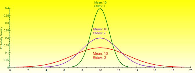
If the distribution can only take a single shape (e.g., Normal distributions are always bell shaped, with the only difference being the central tendency measured by the mean and the spread measured by the standard deviation), then typically only one PDF area chart will be shown with an overlay PDF line chart showing the effects of various parameters on the distribution.

Multiple area charts and line charts will be shown (e.g., Beta distribution) if the distribution can take on multiple shapes (e.g., the Beta distribution is a uniform distribution when alpha = beta = 1; a Parabolic distribution when alpha = beta = 2; a Triangular distribution when alpha = 1 and beta = 2, or vice versa; a positively skewed distribution when alpha = 2 and beta = 5, and so forth).

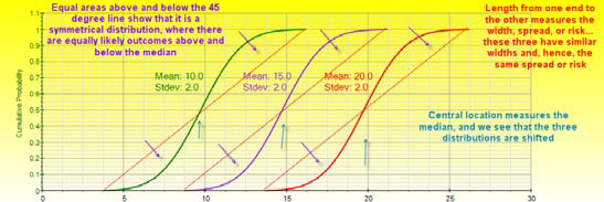
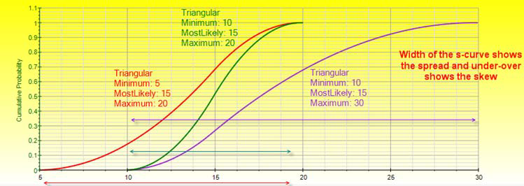
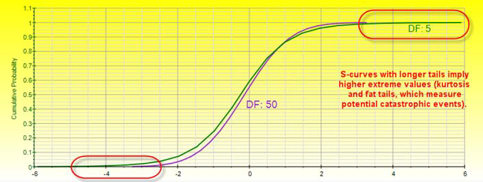
The CDF charts, or S curves, are typically shown as line charts.

The central tendency of a distribution (e.g., the mean and median of a Normal distribution) is its central location.

The starting point of the distribution is sometimes its minimum parameter (e.g., Parabolic, Triangular, Uniform, Arcsine, etc.) or its location parameter (e.g., the Beta distribution’s starting location is 0, but a Beta 4 distribution’s starting point is the location parameter.

The ending point of the distribution is sometimes its maximum parameter (e.g., Parabolic, Triangular, Uniform, Arcsine, etc.) or its natural maximum multiplied by the factor parameter shifted by a location parameter (e.g., the original Beta distribution has a minimum of 0 and maximum value of 1, but a Beta 4 distribution with location = 10 and factor = 2 indicates that the shifted starting point is 10 and ending point is 11, and its width of 1 is multiplied by a factor of 2, which means that the Beta 4 distribution now will have an ending value of 12).

Interactions between parameters are sometimes evident. For example, in the Beta 4 distribution, if the alpha = beta, the distribution is symmetrical, whereas it is more positively skewed the greater the difference between beta – alpha, and the more negatively skewed, the greater the difference between alpha – beta.

Sometimes a distribution’s PDF is shaped by two or three parameters called shape and scale. For instance, the Laplace distribution has two input parameters, alpha location and beta scale, where alpha indicates the central tendency of the distribution (like the mean in a Normal distribution) and beta indicates the spread from the mean (like the standard deviation in a Normal distribution).

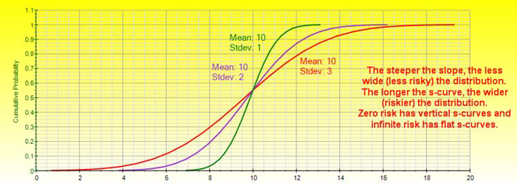
The narrower the PDF, the steeper the CDF S curve looks, and the smaller the width on the CDF curve.

A 45-degree straight line CDF (an imaginary straight line connecting the starting and ending points of the CDF) indicates a Uniform distribution; an S curve CDF with equal amounts above and below the 45-degree straight line indicates a symmetrical and somewhat like a bell- or mound-shaped curve; a CDF completely curved above the 45-degree line indicates a positively skewed distribution, while a CDF completely curved below the 45-degree line indicates a negatively skewed distribution.

A CDF line that looks identical in shape but shifted to the right or left indicates the same distribution but shifted by some location, and a CDF line that starts from the same point but is pulled either to the left or right indicates a multiplicative effect on the distribution such as a factor multiplication.

An almost vertical CDF indicates a high kurtosis distribution with fat tails and where the center of the distribution is pulled up (e.g., see the Cauchy distribution) versus a relatively flat CDF, a very wide and perhaps flat-tailed distribution is indicated.

Some discrete distributions can be approximated by a continuous distribution if its number of trials is sufficiently large and its probabilities of success and failure are fairly symmetrical (e.g., see the Binomial and Negative Binomial distributions). For instance, with a small number of trials and a low probability of success, the Binomial distribution is positively skewed, whereas it approaches a symmetrical Normal distribution when the number of trials is high and the probability of success is around 0.50.

Many distributions are both flexible and interchangeable, e.g., Binomial is Bernoulli repeated multiple times; Arcsine and Parabolic are special cases of Beta; Pascal is a shifted Negative Binomial; Binomial and Poisson approach Normal at the limit; Chi-Square is the squared sum of multiple Normal; Erlang is a special case of Gamma; Exponential is the inverse of the Poisson but on a continuous basis; F is the ratio of two Chi-Squares; Gamma is related to the Lognormal, Exponential, Pascal, Erlang, Poisson, and Chi-Square distributions; Laplace comprises two Exponential distributions in one; the log of a Lognormal approaches Normal; the sum of multiple Discrete Uniforms approach Normal; Pearson V is the inverse of Gamma; Pearson VI is the ratio of two Gammas; PERT is a modified Beta; a large degree of freedom T approaches Normal; Rayleigh is a modified Weibull; and so forth.