QUICK OVERVIEW OF RISK SIMULATOR

• By Admin
• June 16, 2014
• Comments Off on QUICK OVERVIEW OF RISK SIMULATOR

After installing Risk Simulator, start Excel and the Risk Simulator menu will appear in Excel. Risk Simulator comes in 11 languages (English, Chinese Simplified, Chinese Traditional, French, German, Italian, Japanese, Korean, Portuguese, Russian, and Spanish) and has several main modules briefly described below. A wealth of resources are available to get you started including Online Getting Started Videos, User Manuals, Case Studies, White Papers, Help Files, and Hands-on Exercises (these are installed with the software and available on the software DVD, as well on the website www.rovusa.com).

• Monte Carlo Risk Simulation. You can set up probabilistic input Assumptions (45 probability distributions) and output Forecasts, run tens or hundreds of thousands of simulated trials, obtain the resulting probability distributions of your outputs, generate reports, extract simulated data statistics, create scenarios, and generate dynamic charts (histograms, S curves, PDF/CDF charts).
• Forecasting and Prediction Analytics. Using historical data or subject matter estimates, you can run forecast models on time-series or cross-sectional data by applying advanced forecast analytics such as ARIMA, Auto ARIMA, Auto Econometrics, Basic Econometrics, Cubic Splines, Fuzzy Logic, GARCH (8 variations), Exponential J Curves, Logistic S Curves, Markov Chains, Generalized Linear Models (Logit, Probit, Tobit), Multivariate Regressions (Linear and Nonlinear), Neural Network, Stochastic Processes (Brownian Motion, Mean-Reversion, Jump-Diffusion), Time-Series Predictions, and Trendlines.
• Optimization. This module helps you to optimize and find the best Decision variables (which projects to execute, stock portfolio allocation, human resource and budget allocation, pricing levels, and many other applications) subject to Constraints (budget, time, risk, cost, schedule, resources) to minimize or maximize some Objective (profit, risk, revenue, investment return, cost). You can enhance the analysis with Genetic Algorithms, Goal Seek, Efficient Frontier, Dynamic Optimization, and Stochastic Optimization.
• Analytical Tools. These tools are very valuable to analysts working in the realm of risk analysis, from running sensitivity, scenario, and tornado analyses, to distributional fitting to find the best-fitting probability distributions, creating simulation reports and charts, diagnosing data, testing for reliability of your models, computing the exact statistical probabilities of various distributions, finding the statistical properties of your data, testing for precision, and setting correlations among input assumptions.
• ROV BizStats. Comprises over 170 business intelligence and business statistics methods.Types of analysis include Charts (2D/3D Area/Bar/Line/Point, Box-Whisker, Control, Pareto, Q-Q, Scatter); Distributional Fitting (Akaike, Anderson-Darling, Chi-Square, Kolmogorov-Smirnov, Kuiper’s Statistic, Schwarz/Bayes Criterion); Generalized Linear Models (GLM, Logit, Probit, Tobit), Data Diagnostics (Autocorrelation ACF/PACF, Heteroskedasticity, Descriptive Statistics)’ Forecast Prediction (ARIMA, Cubic Spline, Econometrics, Fuzzy Logic, GARCH [E/M/T/GJR], Multiple Regression, J/S Curves, Neural Network,Seasonality Tests, Time-Series Decomposition, Trendlines, Yield Curves); Hypothesis Tests (Parametric T/F/Z, Nonparametric: Friedman’s, Kruskal-Wallis, Lilliefors, Runs, Wilcoxon); and Group Tests (ANOVA, Principal Component Analysis, Segmentation Clustering).
• ROV Decision Tree. This module is used to create and value decision tree models. Additional advanced methodologies and analytics are also included:Decision Tree Models, Monte Carlo Risk Simulation, Sensitivity Analysis, Scenario Analysis, Bayesian (Joint and Posterior Probability Updating), Expected Value of Information, MINIMAX, MAXIMIN, and Risk Profiles.

SIMULATION: QUICK OVERVIEW
Setting up and running a Monte Carlo Risk Simulation in your model simply takes three easy steps: (1) set up a new simulation profile or change/open an existing profile; (2) set input assumptions and output forecasts; and (3) run a simulation and interpret the results. Here are some quick tips about each of these steps as well as additional
options you can set:

• Simulation Profile. Contains Assumptions, Forecasts, Decisions, Constraints, and Objectives and can be set through Risk Simulator |New Profile. Profiles facilitate creating multiple scenarios of simulations. Once a new simulation profile has been created, you can come back later and modify these selections via Risk Simulator | Edit Profile and Risk Simulator | Change Profile.
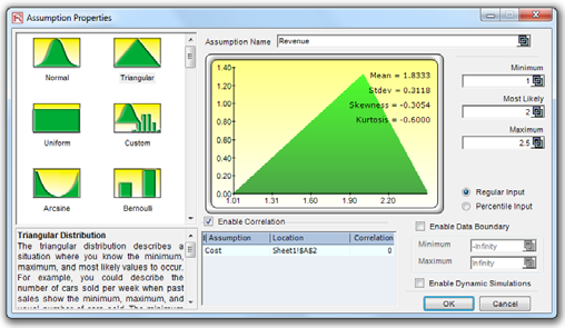
• Input Assumptions. Input Assumptions are assigned to cells without any equations or functions (only cells with simple values or blank cells) using Risk Simulator | Set Input Assumption. Assumptions and forecasts cannot be set unless a simulation profile already exists.
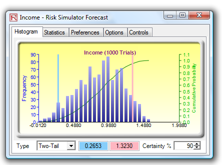
• Output Forecasts. Output forecasts can only be assigned to cells with equations and functions using Risk Simulator | Set Output Forecast. This component tells Risk Simulator which cells to watch out for when running the simulation, such that the results of these cells are saved in computer RAM and used in generating histograms or S curves, running result statistics, extracting simulated data, and other Risk Simulator analytics.
• Seed Value. Slightly different results are produced every time a simulation is run by virtue of the random number generation routine in Monte Carlo simulation. If a seed value is set, the simulation will always yield the same sequence of random numbers, guaranteeing the same final set of results. Set seed values when creating a new profile or editing an existing profile via Risk Simulator | Edit Profile.

• Correlations and Copulas. Set correlations either through Risk Simulator | Tools | Edit Correlations after all the assumptions have been set, or by simply entering the correlations in the Set Assumption dialog (Correlations section) as you go about setting individual assumptions. Correlated assumptions use the Normal Copula, T Copula, and Quasi-Normal Copula algorithms.
• Random Number Generators and Sampling Methods. The Random Number Generator (RNG) is at the heart of any simulation software. The default method is the ROV Risk Simulator proprietary methodology, which provides the best and most robust random numbers. There are 6 supported RNGs (ROV Advanced Subtractive Generator, Subtractive Random Shuffle Generator, Long Period Shuffle Generator, Portable Random Shuffle Generator, Quick IEEE Hex Generator, and Basic Minimal Portable Generator). Also, two sampling methods are available in Risk Simulator: Monte Carlo (default method and typically considered better in most situations) and Latin Hypercube (better only if probabilistic tail events are critical in the simulation). These selections are available in Risk Simulator | Options.
• RS Functions. Simulation statistics (e.g., average, median, standard deviation, skewness, kurtosis, percentile, probability, certainty) can be linked directly in your spreadsheet through the use of Risk Simulator’s RS Functions. Install the RS functions prior to first use at Start | All Programs | Real Options Valuation | Risk Simulator | Tools | Install Functions. Then, in Excel, you can set the functions through clicking on Insert Functions | All and selecting the appropriate RS function to use.
• Precision and Error Control. Precision control takes the guesswork out of estimating the relevant number of trials by allowing the simulation to stop if the level of prespecified precision is reached. As more trials are calculated, the confidence interval narrows and the statistics become more accurate, using the characteristic of confidence intervals to determine when a specified accuracy of a statistic has been reached for each forecast. The specific confidence interval for the precision level can be configured when setting output forecasts at Risk Simulator | Set Output Forecast.
• Truncation, Alternate Parameters, Multidimensional Simulation. Alternate Parameters use percentiles (e.g., 10% and 90%) as an alternate way of inputting assumption parameters instead of the regular inputs such as mean/standard deviation or the more cryptic alpha/beta/gamma. Distribution Truncation enables
  data boundaries in the simulated results. Multidimensional Simulation allows the simulation of uncertain input parameters (i.e., simulating the simulation inputs). These can be configured when setting assumptions at Risk Simulator | Set Input Assumption.
• Run Simulation and Run Super Speed Simulation. Risk Simulator | Run Super Speed Simulation extracts the Excel model into binary relationships and runs the simulation trials in memory at very high speeds. Not all models can run Super Speed (e.g., errors in the model, VBA, or links to external files/models) whereas all models that are set up correctly can run regular speed simulation (Risk Simulator | Run Simulation).

FORECASTING: QUICK OVERVIEW
There are 18 forecast prediction methodologies available in Risk Simulator and they can be assessed though the Risk Simulator | Forecasting menu. Each methodology is briefly discussed below:

• ARIMA. Autoregressive Integrated Moving Average is used for forecasting timeseries data using its own historical data by itself or with exogenous/other variables.
• Auto ARIMA. Runs ARIMA models with the most common settings to test the best-fitting model for time-series data
• Auto Econometrics. Runs some common combinations of Basic Econometrics and returns the best models.
• Basic Econometrics. Applicable for forecasting time-series and cross-sectional data and for modeling relationships among variables, and allows you to create custom multiple regression models.
• Combinatorial Fuzzy Logic. Applies fuzzy logic algorithms for forecasting time series data by combining other forecast methods to create an optimized model.
• Cubic Spline Curves.Interpolates missing values of a time-series data set and extrapolates values of future forecast periods using nonlinear curves.
• Custom Distributions. Expert opinions can be collected and a customized distribution can be generated. This forecasting technique comes in handy when the data set is small or the goodness of fit is bad when applied to a distributional fitting routine, and can be accessed through Risk Simulator | Set Input Assumption | Custom Distribution.
• GARCH.The Generalized Autoregressive Conditional Heteroskedasticity model is used to model historical and forecast future volatility levels of a time-series of raw price levels of a marketable security (e.g., stock prices, commodity prices, and oil prices). GARCH first converts the prices into relative returns, and then runs an internal optimization to fit the historical data to a mean-reverting volatility term structure, while assuming that the volatility is heteroskedastic in nature (changes over time according to some econometric characteristics). Several variations of this methodology are available in Risk Simulator, including EGARCH, EGARCH-T, GARCH-M, GJR-GARCH, GJR-GARCH-T, IGARCH, and T-GARCH.
• J Curve. This function models exponential growth where value of the next period depends on the current period’s level and the increase is exponential. Over time, the values will increase significantly from one period to another. This model is typically used in forecasting biological growth and chemical reactions over time.
• Markov Chain. Models the probability of a future state that depends on a previous state, forming a chain when linked together that reverts to a long-run steady state level. It is typically used to forecast the market share of two competitors.
• Maximum Likelihood/Generalized Linear Models (Logit, Probit, Tobit). Generalized Linear Models (GLM) are used to forecast the probability of something occurring given some independent variables (e.g., predicting if a credit line will default given the obligor’s characteristics such as age, salary, credit card debt levels, or the probability a patient will have lung cancer based on age and number of cigarettes smoked monthly, and so forth). The dependent variable is limited (i.e., binary 1 and 0 for default/cancer, or limited to integer values 1, 2, 3, etc.). Traditional regression analysis will not work as the predicted probability is usually less than zero or greater than one, and many of the required regression assumptions are violated (e.g., independence and normality of the errors).
• Multivariate Regression. Multivariate regression is used to model the relationship structure and characteristics of a certain dependent variable as it depends on other independent exogenous variables. Using the modeled relationship, we can forecast the future values of the dependent variable. The accuracy and goodness of fit for this model can also be determined. Linear and nonlinear models can be fitted in the multiple regression analysis.
• Neural Network. Often used to refer to a network or circuit of biological neurons, modern usage of the term often refers to artificial neural networks comprising artificial neurons, or nodes, recreated in a software environment. Suchnetworks attempt to mimic the neurons in the human brain in ways of thinking and identifying patterns and, in our situation, identifying patterns for the purposes of forecasting time-series data.
• Nonlinear Extrapolation. The underlying structure of the data to be forecasted is assumed to be nonlinear over time. For instance, a data set such as 1, 4, 9, 16, 25 is considered to be nonlinear (these data points are from a squared function).
• S Curve. The S curve, or logistic growth curve, starts off like a J curve, with exponential growth rates. Over time, the environment becomes saturated (e.g., market saturation, competition, overcrowding), the growth slows, and the forecast value eventually ends up at a saturation or maximum level. This model is typically used in forecasting market share or sales growth of a new product from market introduction until maturity and decline, population dynamics, and other naturally occurring phenomenon.
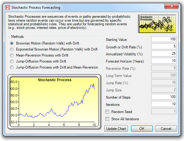
• Stochastic Processes. Sometimes variables cannot be readily predicted using traditional means, and these variables are said to be stochastic. Nonetheless, most financial, economic, and naturally occurring phenomena (e.g., motion of molecules through the air) follow a known mathematical law or relationship. Although the resulting values are uncertain, the underlying mathematical structure is known and can be simulated using Monte Carlo risk simulation. The processes supported include Brownian motion random walk, mean-reversion, jump-diffusion, and mixed processes, useful for forecasting non stationary time-series variables.
• Time-Series Analysis and Decomposition. In well-behaved time-series data (e.g., sales revenues and cost structures of large corporations), the values tend to have up to three elements: a base value, trend, and seasonality. Time-series analysis uses these historical data and decomposes them into these three elements, and recomposes them into future forecasts. In other words, this forecasting method, like some of the others described, first performs a back-fitting (backcast) of historical data before it provides estimates of future values (forecasts).
• Trendlines. Trendlines can be used to determine if a set of time-series data follows any appreciable trend. Trends can be linear or nonlinear (such as exponential, logarithmic, moving average, power, or polynomial).

OPTIMIZATION: QUICK OVERVIEW
In most simulation models, there are variables over which you have control, such as how much to charge for a product, how much to invest in a project, or which projects to select or invest in, all the while being subject to some Constraints or limitations (e.g., budget, time, schedule, cost, and resource constraints). These controlled variables are called Decision variables. Finding the optimal values for decision variables can make the difference between reaching an important goal or Objective and missing that goal. These OCD variables have to be set up via the Risk Simulator | Optimization menu before an optimization can be run.

• Objective. The output we care about that we wish to Maximize (profits, revenue, returns, etc.) or Minimize (e.g., cost, risk, etc.).
• Decisions. The variables you have control over and that can be continuous (e.g., % budget allocation), binary (e.g., go or no-go on projects), or discrete integers (e.g., number of light bulbs to manufacture).
• Constraints. Limitations in the model, such as budget, time, schedule, or other resource constraints.
• Efficient Frontier. The Efficient Frontier optimization procedure applies the concepts of marginal increments and shadow pricing in optimization. That is, what would happen to the results of the optimization if one of the constraints were relaxed slightly? This is the concept of the Markowitz efficient frontier in investment finance.
• Static Optimization. Risk Simulator can be used to run a Static Optimization, that is, an optimization that is run on a static model, where no simulations are runand all the inputs in the model are static and unchanging, and it is applicable when it is assumed that no uncertainties exist. A static optimization is often run first to determine if there exist solutions to the optimization problem before a more protracted analysis is performed.
• Dynamic Optimization. Monte Carlo simulation is first run and the results of the simulation are applied in the model, then optimization is run (e.g., Simulation- Optimization). A simulation is run for N trials, and then an optimization process is run for M iterations until the optimal results are obtained or an infeasible set is found. You can choose which forecast and assumption statistics to use and replace in the model after the simulation is run. Then, these forecast statistics can be applied in the optimization process.
• Stochastic Optimization. This is similar to the dynamic optimization procedure where the entire dynamic optimization process is repeated T times: A simulation with N trials is run, and then an optimization is run with M iterations to obtain the optimal results. Then the process is replicated T times. The results will be a forecast chart of each decision variable with T values, indicating the range of the optimal decision variables.
• Genetic Algorithm. A type of evolutionary algorithms that generates solutions to optimization problems using techniques inspired by natural evolution, such as inheritance, mutation, selection, and crossover. Genetic Algorithm is a search heuristic that mimics the process of natural evolution and is routinely used to generate useful solutions to optimization and search problems.
• Goal Seek. A search algorithm applied to find the solution of a single variable within a model. Used if you know the result that you want from a formula or a model, but are not sure what input value the formula needs to get that result.
• Conditional Means, Percentiles Statistics, Search Algorithms, and Super Speed Dynamic/Stochastic Optimization. Percentiles, Statistics, and Conditional Means are some additional statistics for stochastic optimization, including percentiles as well as conditional means, which are critical in computing Conditional Value at Risk measures. Super Speed Simulation in Dynamic and Stochastic Optimization runs simulations at super speed while integrated with optimization.

ROV BIZSTATS: QUICK OVERVIEW

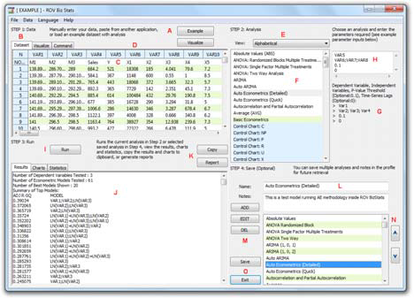
• Step 1: Data. Run ROV BizStats at Risk Simulator | ROV BizStats and click on Example to load a sample data and model profile, or type in your data, or copy/paste your existing data into the data grid.
• Step 2: Analysis. Select the relevant model to run and using the example data input settings, enter in the relevant variables. Separate variables for the same parameter using semicolons and use a new line (hit Enter to create a new line) for different parameters.
• Step 3: Run. Computes the results. You can view any relevant analytical results, charts, or statistics from the various results tabs.
• Step 4: Save (Optional). If required, you can provide a model name to save the existing model. Multiple models can be saved in the same profile. Existing models can be edited or deleted, or rearranged in order of appearance, and all the changes can be saved into a single profile with the file name extension *.bizstats.

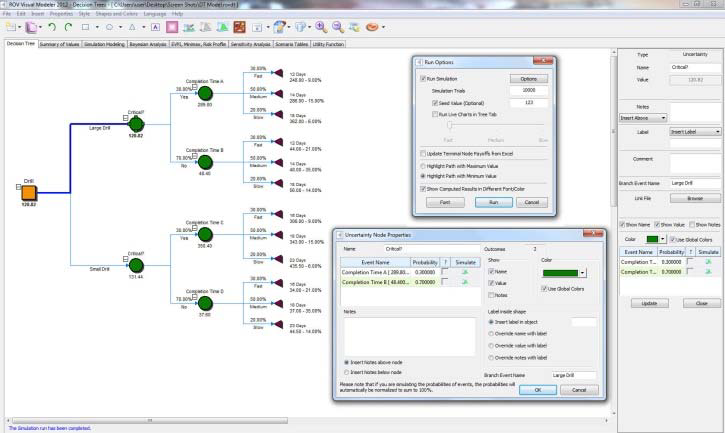
ROV DECISION TREE: QUICK OVERVIEW

• Decision Tree. This is the main tab of the ROV Decision Tree, used to create and value decision tree models. You can very quickly draw a decision tree complete with Decision Variables (square), Uncertainty Events (circle), and Terminal Nodes (triangles). You can also change the properties of these shapes (color, font, labels, size, connection lines), create and save your own styles, and set single point input values or set simulation assumptions in the uncertainty and terminal event nodes.
• Summary of Values. This tab summarizes all the single point input values set previously on the decision tree in a simple layout.
• Monte Carlo Risk Simulation. Runs Monte Carlo Risk Simulation on the decision tree. It allows you to set probability distributions as input assumptions for running simulations. You can either set an assumption for the selected node or set a new assumption and use this new assumption (or use previously created assumptions) in a numerical equation or formula.
• Bayesian Analysis. Used on any two uncertainty events that are linked along a path, and computes the joint, marginal, and Bayesian posterior updated probabilities by entering the prior probabilities and reliability conditional probabilities; or reliability probabilities can be computed when you have posterior updated conditional probabilities.
• EVPI, Minimax, Risk Profile. Computes the Expected Value of Perfect Information (EVPI) and MINIMAX and MAXIMIN Analysis, as well as the Risk Profile and the Value of Imperfect Information.
• Sensitivity Analysis. Sensitivity analysis is run on the input probabilities todetermine the impact of inputs on the values of decision paths.
• Scenario Tables. Generates scenario tables to determine the output values given some changes to the input.
• Utility Functions. Utility functions, or U(x), are sometimes used in place of expected values of terminal payoffs in a decision tree. They can be modeled for a decision maker who is risk-averse (downsides are more disastrous or painful than an equal upside potential), risk-neutral (upsides and downsides have equal attractiveness), or risk-loving (upside potential is more attractive).

ANALYTICAL TOOLS: QUICK OVERVIEW

• Check Model. After a model is created and after assumptions and forecasts have been set, you can run the simulation as usual or run the Check Model tool to test if the model has been set up correctly. While this tool checks for the most common model problems as well as for problems in Risk Simulator assumptions and forecasts, it is in no way comprehensive enough to test for all types of problems. It is still up to the model developer to make sure the model works properly.
• Create Forecast Statistics Table. After a simulation is run, you can extract the output forecasts’ main statistics as a comprehensive table.
• Create Report. After a simulation is run, you can generate a report of the assumptions and forecasts used in the simulation run, as well as the results obtained during the simulation run.
• Data Deseasonalization and Detrending. Removes any seasonal and trending components in your original data.
• Data Extraction. A simulation’s raw data can be very easily extracted using Risk Simulator’s Data Extraction routine. Both assumptions and forecasts can be extracted, but a simulation must first be run. Data from simulated input assumptions and forecast outputs can be extracted in Excel as a new worksheet, as a text file, or as a *.risksim file, where the latter can be opened as dynamic forecast charts later on.
• Data Open/Import. Opens the saved *.risksim files as dynamic forecast charts.
• Diagnostic Tool. Determines the econometric properties of your data. The diagnostics include checking the data for heteroskedasticity, nonlinearity, outliers, specification errors, micronumerosity, stationarity and stochastic properties, normality and sphericity of the errors, and multicollinearity. Each test is described in more detail in its respective report in the model.
• Distributional Analysis. Computes the probability density function (PDF), where given some distribution and its parameters, you can determine the probability of occurrence given some outcome x. The cumulative distribution function (CDF) is also computed, which is the sum of the PDF values up to this x value. Finally, the inverse cumulative distribution function (ICDF) is used to compute the value x given the cumulative probability of occurrence. Works for all 45 probability distributions available in Risk Simulator.
• Distributions Charts and Tables. Used to compare different parameters of the same distribution (e.g., the shapes and PDF, CDF, ICDF values of a Weibull distribution with Alpha and Beta of [2, 2], [3, 5], and [3.5, 8]) and overlays them on top of one another.
• Distributional Designer. Allows you to create custom distributions by entering or pasting in existing data. Data can be in a single column or two columns (unique values and their respective frequencies such that the probabilities of occurrence sum to 100%).
• Distributional Fitting (Single Variable). Determines which distribution to use for a particular input variable in a model and the relevant distributional parameters. Advanced algorithms are employed such as Akaike Information Criterion,Anderson-Darling, Chi-Square, Kolmogorov-Smirnov, Kuiper’s Statistic, and Schwarz/Bayes Information Criterion.
• Distributional Fitting (Multi-Variable).Runs distributional fitting on multiple variables at once, and captures their correlations as well as computing the relevant statistical significance of the correlations and the fit.
• Distributional Fitting (Percentiles). Uses an alternate method of entry (percentiles and first/second moment combinations) to find the best-fitting parameters of a specified distribution without the need for having raw data. This method is suitable for use when there are insufficient data, when only percentiles and moments are available, or as a means to recover the entire distribution with only two or three data points but the distribution type needs to be assumed or known.
• Edit Correlations. Sets up a correlation matrix by manually entering or pasting from Windows clipboard (ideal for large correlation matrices and multiple correlations), but only after assumptions have all been set.
• Hypothesis Testing. Tests the means and variances of two distributions to determine if they are statistically identical or statistically different from one another; that is, whether the differences are based on random chance or if they are, in fact, statistically significant.
• Nonparametric Bootstrap. Estimates the reliability or accuracy of forecast statistics or other sample raw data, and analyzes sample statistics empirically by repeatedly sampling the data and creating distributions of the different statistics from each sampling. Essentially, bootstrap simulation is used in hypothesis testing.
• Overlay Charts. Used to compare different distributions (theoretical input assumptions and empirically simulated output forecasts) and to overlay them on top of one another for a visual comparison.
• Principal Component Analysis. Identifies patterns in data and recasts the data in such a way as to highlight their similarities and differences. Patterns of data are very difficult to find in high dimensions when multiple variables exist, and higher dimensional graphs are very difficult to represent and interpret. Once the patterns in the data are found, they can be compressed, and the number of dimensions is reduced.
• Scenario Analysis. Run multiple scenarios of your existing model quickly and effortlessly by changing one or two input parameters to determine the output of a variable.
• Seasonality Test. Many time-series data exhibit seasonality where certain events repeat themselves after some time period or seasonality period (e.g., ski resorts’ revenues are higher in winter than in summer, and this predictable cycle will repeat itself every winter).
• Segmentation Clustering. From an original data set, algorithms (combination k-means hierarchical clustering and other method of moments) are run to find the best-fitting groups or natural statistical clusters to statistically divide, or segment, the original data set into different groups or segments.
• Sensitivity Analysis. While tornado analysis (tornado charts and spider charts) applies static perturbations before a simulation run, sensitivity analysis applies dynamic perturbations created after the simulation run.
• Statistical Analysis. Determines the statistical properties of the data. The diagnostics run include checking the data for various statistical properties, from basic descriptive statistics to testing for and calibrating the stochastic properties of the data.
• Structural Break Test. A time-series data set is divided into two subsets and the algorithm is used to test each subset individually and on one another and on the entire data set to statistically determine if, indeed, there is a break starting at a particular time period.
• Tornado Analysis. A powerful simulation tool that captures the static impacts of each variable on the outcome of the model. That is, the tool automatically perturbs each variable in the model a preset amount, captures the fluctuation on the model’s forecast or final result, and lists the resulting perturbations ranked from the most significant to the least.

PROBABILITY DISTRIBUTIONS: QUICK OVERVIEW
There are 45 probability distributions available in Risk Simulator, and the most commonly used probability distributions are listed here in order of popularity of use. See the user manual for technical details on all 45 distributions.

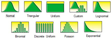
• Normal. The most important distribution in probability theory, it describes many natural phenomena (people’s IQ or height, inflation rate, future price of gasoline, etc.). The uncertain variable could as likely be above the mean as it could be below the mean (symmetrical about the mean), and the uncertain variable is more likely to be in the vicinity of the mean than further away. Mean (μ) 0 and standard deviation (σ) > 0.
• Triangular. The minimum, maximum, and most likely values are known from past data or expectations. The distribution forms a triangular shape, which shows that values near the minimum and maximum are less likely to occur than those near the most-likely value. Minimum ≤ Most Likely ≤ Maximum, but all three cannot have identical values.
• Uniform. All values that fall between the minimum and maximum occur with equal likelihood and the distribution is flat. Minimum < Maximum.
• Custom. The custom nonparametric simulation is a data-based empirical distribution in which available historical or comparable data are used to define the custom distribution, and the simulation is distribution-free and, hence, does not require any input parameters (nonparametric). This means that we let the data define the distribution and do not explicitly force any distribution on the data. The data is sampled with replacement repeatedly using the Central Limit Theorem.
• Lognormal. Used in situations where values are positively skewed, for example, in financial analysis for security valuation or in real estate for property valuation, and where values cannot fall below zero (e.g., stock prices and real estate prices are usually positively skewed rather than normal or symmetrically distributed and cannot fall below the lower limit of zero but might increase to any price without limit). Mean (μ) <=> 0 and standard deviation (σ) > 0.
• Binomial. Describes the number of times a particular event occurs in a fixed number of trials, such as the number of heads in 10 flips of a coin or the number of defective items out of 50 items chosen. For each trial, only two mutually exclusive outcomes are possible, and the trials are independent, where what happens in the first trial does not affect the next trial. The probability of an event occurring remains the same from trial to trial. Probability of success (P) > 0 and the number of total trials (N) is a positive integer.
• Discrete Uniform. Known as the equally likely outcomes distribution, where the distribution has a set of N elements, then each element has the same probability, creating a flat distribution. This distribution is related to the uniform distribution but its elements are discrete and not continuous. Min < Max, and both are integers.
• Poisson. Describes the number of times an event occurs in a given interval, such as the number of telephone calls per minute or the number of errors per page in a document. The number of possible occurrences in any interval is unlimited and the occurrences are independent. The number of occurrences in one interval does not affect the number of occurrences in other intervals, and the average number of occurrences must remain the same from interval to interval. Lambda (Average Rate) > 0 but ≤ 1000.
• Exponential. Widely used to describe events recurring at random points in time, for example, the time between events such as failures of electronic equipment or the time between arrivals at a service booth. It is related to the Poisson distribution, which describes the number of occurrences of an event in a given interval of time. An important characteristic of the exponential distribution is its memory less property, which means that the future lifetime of a given object has the same distribution regardless of the time it existed. In other words, time has no effect on future outcomes. Success rate (λ) > 0.