Stochastic Forecasting
- By Admin
- November 28, 2014
- Comments Off on Stochastic Forecasting
Theory
A stochastic process is nothing but a mathematically defined equation that can create a series of outcomes over time, outcomes that are not deterministic in nature; that is, an equation or process that does not follow any simple discernible rule such as price will increase X% every year or revenues will increase by this factor of X plus Y%. A stochastic process is by definition nondeterministic, and one can plug numbers into a stochastic process equation and obtain different results every time. For instance, the path of a stock price is stochastic in nature, and one cannot reliably predict the exact stock price path with any certainty. However, the price evolution over time is enveloped in a process that generates these prices. The process is fixed and predetermined, but the outcomes are not. Hence, by stochastic simulation, we create multiple pathways of prices, obtain a statistical sampling of these simulations, and make inferences on the potential pathways that the actual price may undertake given the nature and parameters of the stochastic process used to generate the time series. Four stochastic processes are included in Risk Simulator’s Forecasting tool, including Geometric Brownian motion or random walk, which is the most common and prevalently used process due to its simplicity and wide-ranging applications. The other three stochastic processes are the mean-reversion process, jump-diffusion process, and a mixed process.
The interesting thing about stochastic process simulation is that historical data is not necessarily required; that is, the model does not have to fit any sets of historical data. Simply compute the expected returns and the volatility of the historical data or estimate them using comparable external data, or make assumptions about these values.
Procedure
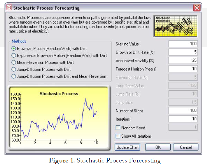
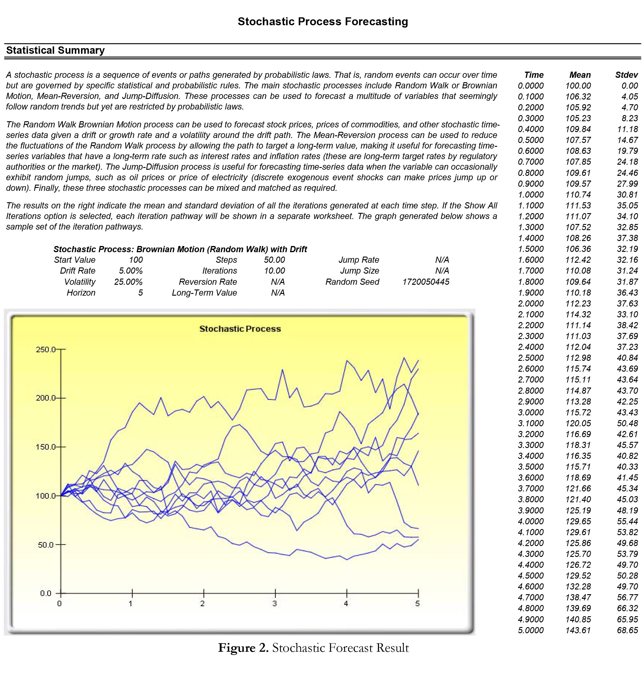
Results Interpretation
Figure 2 shows the results of a sample stochastic process. The chart shows a sample set of the iterations while the report explains the basics of stochastic processes. In addition, the forecast values (mean and standard deviation) for each time period is provided. Using these values, you can decide which time period is relevant to your analysis and set assumptions based on these mean and standard deviation values using the normal distribution. These assumptions can then be simulated in your own custom model.
Notes
Brownian Motion Random Walk Process
The Brownian motion random walk process takes the form of
Error! Objects cannot be created from editing field codes.
for regular options simulation, or a more generic version takes the form of
Error! Objects cannot be created from editing field codes.
for a geometric process.
For an exponential version, we simply take the exponentials, and as an example, we have
Error! Objects cannot be created from editing field codes.
where we define
S as the variable’s previous value
δS as the change in the variable’s value from one step to the next
µ as the annualized growth or drift rate
σ as the annualized volatility
To estimate the parameters from a set of time-series data, the drift rate and volatility can be found by setting µ to be the average of the natural logarithm of the relative returns
Error! Objects cannot be created from editing field codes.
while σ is the standard deviation of all

values.
Mean-Reversion Process
The following describes the mathematical structure of a mean-reverting process with drift:
Error! Objects cannot be created from editing field codes.
To obtain the rate of reversion and long-term rate, using the historical data points, run a regression such that
Error! Objects cannot be created from editing field codes.
and we find
Error! Objects cannot be created from editing field codes. and Error! Objects cannot be created from
editing field codes.
where we define
η as the rate of reversion to the mean
Error! Objects cannot be created from editing field codes. as the long-term value the process reverts to
Y as the historical data series
β as the intercept coefficient in a regression analysis
β as the slope coefficient in a regression analysis
Jump Diffusion Process
A jump diffusion process is similar to a random walk process but there is a probability of a jump at any point in time. The occurrences of such jumps are completely random but its probability and magnitude are governed by the process itself as introduced below.
for a jump diffusion process
Error! Objects cannot be created from editing field codes.
where we define
0 as the jump size of S
F(λ) as the inverse of the Poisson cumulative probability distribution
λ as the jump rate of S
The jump size can be found by computing the ratio of the postjump to the prejump levels, and the jump rate can be imputed from past historical data. The other parameters are found the same way as above.

Recent Comments