TECHNICAL ISSUES IN CORRELATIONS

• By Admin
• April 8, 2015
• Comments Off on TECHNICAL ISSUES IN CORRELATIONS

• The following lists some key correlation effects and details that will be helpful in modeling:
  • Correlation coefficients range from –1.00 to +1.00, with 0.00 as a possible value. Typically, when we use the term correlation, we usually mean a linear correlation.
  • The correlation coefficient has two parts: a sign and a value. The sign shows the directional relationship whereas value shows the magnitude of the effect (the higher the value, the higher the magnitude, while zero values imply no relationship). Another way to think of a correlation’s magnitude is the inverse of noise (the lower the value, the higher the noise).
  • Correlation implies dependence and does not imply causality. Two completely unrelated random variables might display some correlation, but this does not imply any causation between the two (e.g., sunspot activity and events in the stock market are correlated, but there is no causation between the two). In other words, if two variables are correlated, it simply means both variables move together in the same or opposite direction (positive versus negative correlations) with some strength of co‐movements. It does not, however, imply that one variable causes another. In addition, one cannot determine the exact impact or how much one variable causes another to move.
  • If two variables are independent of one another, correlation will be, by definition, zero. However, a zero correlation may not imply independence (because there might be some nonlinear relationships).
  • Correlations can be visually approximated on an X‐Y plot (see Figures 5.51 and 5.52 in Dr. Johnathan Mun’s Modeling Risk, Third Edition, for some examples). If we generate an X‐Y plot and the line is flat, the correlation is close to or equal to zero; if the slope is positive (data slopes upward), then the correlation is positive; if the slope is negative (data slopes downward), then the correlation is negative; the closer the scatter plot’s data points are to a straight line, the higher the linear correlation value.
  • Figure 3 illustrates a few scatter charts with a pairwise X and Y variables (e.g., hours of study and school grades). If we draw an imaginary best‐fitting line in the scatter diagram, we can see the approximate correlation (we will show a computation of correlation in a moment, but for now, let’s just visualize). Part A shows a relatively high positive correlation coefficient (R) of about 0.7 as an increase in X means an increase in Y, so there is a positive slope and therefore a positive correlation. Part B shows an even stronger negative correlation (negatively sloped, an increase of X means a decrease of Y and vice versa). It has slightly higher magnitude because the dots are closer to the line. In fact, when the dots are exactly on the line, as in Part D, the correlation is +1 (if positively sloped) or –1 (if negatively sloped), indicating a perfect correlation. Part C shows a situation where the curve is perfectly flat, or has zero correlation, where, regardless of the X value, Y remains unchanged, indicating that there is no relationship. These are all very basic and good. The problem arises when there are nonlinear relationships (typically the case in a many real‐life situations) as shown in Figure 4. Part E shows an exponential relationship between X and Y. If we use a nonlinear correlation, we get +0.9, but if we use a linear correlation, it is much lower at 0.6 (Part F), which means that there is information that is not picked up by the linear correlation. The situation gets a lot worse when we have a sinusoidal relationship, as in Parts G and H. The nonlinear correlation picks up the relationship very nicely with a 0.9 correlation coefficient; using a linear correlation, the best‐fitting line is literally a flat horizontal line, indicating zero correlation. However, just looking at the picture would tell you that there is a relationship. So, we must therefore distinguish between linear and nonlinear correlations, because correlation affects risk, and we are dealing with risk analysis.
  • The population correlation coefficient (ρ) can be defined as the standardized covariance:
    
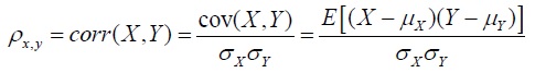
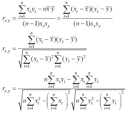
    where X and Y are the data from two variables’ population. The covariance measures the average or expectation (E) of the co-movements of all X values from its mean (μx) multiplied by the co‐movements of all Y values from its population mean(μy). The value of covariance is between negative and positive infinity, making its interpretation fairly difficult. However, by standardizing the covariance through dividing it by the population standard deviation (σ) of X and Y, we obtain the correlation coefficient, which is bounded between –1.00 and +1.00
  • However, in practice, we typically only have access to sample data and the sample correlation coefficient (r) can be determined using the sample data from two variables x and y, their averages ( x, y ), their standard deviations (sx,sy), and the count of x and y data pairs:
    
  • Correlations are symmetrical. In other words, the rA,B = rB,A. Therefore, we sometimes call
    correlation coefficients pairwise correlations
  • If there are n variables, then the number of total pairwise correlation is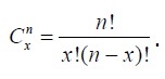For example, if there are 3 variables, A, B, C, the number of pairwise (x = 2, or two items are chosen at a time) combinations total
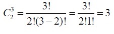
  • Correlations can be linear or nonlinear. Pearson’s product moment correlation coefficient is used to model linear correlations and Spearman’s rank‐based correlation is used to model nonlinear correlations.
  • Linear correlations (also known as the Pearson’s R) can be computed using Excel’s CORREL function or using the equations described previously.
  • Nonlinear correlations are computed by first ranking the nonlinear raw data, and then applying the linear Pearson’s correlation. The result is a nonlinear rank correlation or Spearman’s R. Use the correlation version (linear or nonlinear) that has a higher absolute value.
  • There are two general types of correlations: parametric and nonparametric correlations. Pearson’s correlation coefficient is the most common correlation measure, and is usually referred to simply as the correlation coefficient. However, Pearson’s correlation is a parametric measure, which means that it requires both correlated variables to have an underlying normal distribution and that the relationship between the variables is linear. When these conditions are violated, which is often the case in Monte Carlo simulation, the nonparametric counterparts become more important. Spearman’s rank correlation and Kendall’s tau are the two nonparametric alternatives. The Spearman correlation is most commonly used and is most appropriate when applied in the context of Monte Carlo simulation––there is no dependence on normal distributions or linearity, meaning that correlations between different variables with different distribution can be applied. In order to compute the Spearman correlation, first rank all the x and y variable values and then apply the Pearson’s correlation computation. In the case of Risk Simulator, the correlation used is the more robust nonparametric Spearman’s rank correlation. However, to simplify the simulation process, and to be consistent with Excel’s correlation function, the correlation inputs required are the Pearson’s correlation coefficient. Risk Simulator will then apply its own algorithms to convert them into Spearman’s rank correlation, thereby simplifying the process. However, to simplify the user interface, we allow users to enter the more common Pearson’s product‐moment correlation (e.g., computed using Excel’s CORREL function), while in the mathematical codes, we convert these simple correlations into Spearman’s rank‐based correlations for distributional simulations.
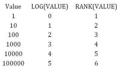
  • The approach to Spearman’s nonlinear correlation is very simple. Using the original data we first “linearize” the data and then apply the Pearson’s correlation computation to get the Spearman’s correlation. Typically, whenever there is nonlinear data, we can linearize it by either using a LOG function (or equivalently, an LN or natural log function) or a RANK function. The table below illustrates this effect. The original value is clearly nonlinear (it is 10x where x is from 0 to 5). However, if you apply a log function, the data becomes linear (1, 2, 3, 4, 5) or when you apply ranks, the rank (either high to low or low to high) is also linear. Once we have linearized the data, we can apply the linear Pearson’s correlation. To summarize, Spearman’s nonparametric nonlinear correlation coefficient is obtained by first ranking the data and then applying Pearson’s parametric linear correlation coefficient.
  • The square of the correlation coefficient (R) is called the coefficient of determination or Rsquared. This is the same R‐squared used in regression modeling, and it indicates the percentage variation in the dependent variable that is explained given the variation in the independent variable(s).
  • R‐squared is limited to be between 0.00 and 1.00, and is usually shown as a percent. Specifically, as R has a domain between –1.00 and +1.00, squaring either a positive or negative R value will always yield a positive R‐squared value, and squaring any R value between 0.00 and 1.00 will always yield an R‐squared result between 0.00 and 1.00. This means that R‐squared is localized to between 0% and 100% by construction.
  • In a simple positively related model, negative correlations reduce total portfolio risk, whereas positive correlations increase total portfolio risk. Conversely, in a simple negatively related model, negative correlations increase total portfolio risk, whereas positive correlations decrease total portfolio risk.
    • Positive Model (+) with Positive Correlation (+) = Higher Risk (+).
    • Positive Model (+) with Negative Correlation (–) = Lower Risk (–).
    • Negative Model (–) with Positive Correlation (+) = Lower Risk (–).
    • Negative Model (–) with Negative Correlation (–) = Higher Risk (+).
  • Portfolio Diversification typically implies the following condition: Positive Model (+) with Negative Correlation (–) = Lower Risk (–). For example, the portfolio level’s (p) diversified risk is computed by taking
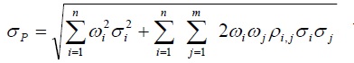    where ωi,j are the respective weights or capital allocation across each project;ρi,j are the respective cross‐correlations between the assets, and σi,j are the volatility risks. Hence, if the cross‐correlations are negative, there are risk diversification effects, and the portfolio risk decreases.
  • Examples of a simple positively related model are an investment portfolio (the total of the returns in a portfolio is the sum of each individual asset’s returns, i.e., A + B + C = D, therefore, increase A or B or C, and the resulting D will increase as well, indicating a positive directional relationship) or the total of the revenues of a company is the sum of all the individual products’ revenues. Negative correlations in such models mean that if one asset’s returns decrease (losses), another asset’s returns would increase (profits). The spread or distribution of the total net returns for the entire portfolio would decrease (lower risk). The negative correlation would, therefore, diversify the portfolio risk.
  • Alternatively, an example of a simple negatively related model is revenue less cost equals net income (i.e., A – B = C, which means that as B increases, C would decrease, indicating a negative relationship). Negatively correlated variables in such a model would increase the total spread of the net income distribution
  • In more complex or larger models where the relationship is difficult to determine (e.g., in a discounted cash flow model where we have revenues of one product being added to revenues of other products but less costs to obtain the gross profits, and where depreciation is used as tax shields, then taxes are deducted, etc.), and both positive and negative correlations may exist between the various revenues (e.g., similar product lines versus competing product lines cannibalizing each other’s revenues), the only way to determine the final effect is through simulations.
  • Although the computations required to correlate variables in a simulation is complex, the resulting effects are fairly clear. Figure 1 shows a simple correlation model (Correlation Effects Model in the example folder). The calculation for revenue is simply price multiplied by quantity.The same model is replicated for no correlations, positive correlation (+0.9), and negative correlation (–0.9) between price and quantity. The resulting statistics are shown in Figure 2. Notice that the standard deviation of the model without correlations is 0.1450, compared to 0.1886 for the positive correlation, and 0.0717 for the negative correlation. That is, for simple models, negative correlations tend to reduce the average spread of the distribution and create a tight and more concentrated forecast distribution as compared to positive correlations with larger average spreads. However, the mean remains relatively stable. This result implies that correlations do little to change the expected value of projects but can reduce or increase a project’s risk.
    • The resulting simulation statistics indicate that the negatively correlated variables provide a tighter or smaller standard deviation or overall risk level on the model. This relationship exists because negative correlations provide a diversification effect on the variables and, hence, tend to make the standard deviation slightly smaller. Thus, we need to make sure to input correlations when there indeed are correlations between variables. Otherwise this interacting effect will not be accounted for in the simulation.
    • The positive correlation model has a larger standard deviation because a positive correlation tends to make both variables travel in the same direction, making the extreme ends wider and, hence, increases the overall risk. Therefore, the model without any correlations will have a standard deviation between the positive and negative correlation models.
    • Notice that the expected value or mean does not change much. In fact, if sufficient simulation trials are run, the theoretical and empirical values of the mean remain the same. The first moment (central tendency or expected value) does not change with correlations. Only the second moment (spread or risk and uncertainty) will change with correlations (Figure 3).
    • Note that this characteristic exists only in simple models with a positive relationship. That is, a Price × Quantity model is considered a “positive” relationship model (as are Price + Quantity), where a negative correlation decreases the range and a positive correlation increases the range. The opposite is true for negative relationship models. For instance, Price / Quantity or Price – Quantity would be a negative relationship model, where a positive correlation will reduce the range of the forecast variable, and a negative correlation will increase the range. Finally, for more complex models (e.g., larger models with multiple variables interacting with positive and negative relationships and sometimes with positive and negative correlations), the results are hard to predict and cannot be determined theoretically. Only by running a simulation can the true results of
      the range and outcomes be determined. In such a scenario, Tornado Analysis and Sensitivity Analysis would be more appropriate.
  • Correlations typically affect only the second moment (risk) of the distribution, leaving the first
    moment (mean or expected returns) relatively stable. There is an unknown effect on the third and fourth moments (skew and kurtosis), and only after a simulation is run can the outcomes be empirically determined because the effects are wholly dependent on the distributions’ type, skew, kurtosis, and shape. Therefore, in traditional single point estimates where only the first moment is determined, correlations will not affect the results. When simulation models are used, the entire probability distribution of the results are obtained and, hence, correlations are critical.
  • Correlations should be used in a simulation if there are historical data to compute its value. Even in situations without historical data but with clear theoretical justifications for correlations, one should still input them. Otherwise the distributional spreads would not be accurate. For instance, a demand curve is theoretically negatively sloped (negatively correlated), where the higher the price, the lower the quantity demanded (due to income and substitution effects) and vice versa. Therefore, if no correlations are entered in the model, the simulation results may randomly generate high prices with high quantity demanded, creating extreme high revenues, as well as low prices and low quantity demanded, creating extreme low revenues. The simulated probability distribution of revenues would, hence, have wider spreads into the left and right tails. These wider spreads are not representative of the true nature of the distribution. Nonetheless, the mean or expected value of the distribution remains relatively stable. It is only the percentiles and confidence intervals that get biased in the model.
  • Therefore, even without historical data, if we know that correlations do exist through experimentation, widely accepted theory, or even simply by logic and guesstimates, one should still input approximate correlations into the simulation model. This approach is acceptable because the first moment or expected values of the final results will remain unaffected (only the risks will be affected as discussed). Typically, the following approximate correlations can be applied even without historical data:
    • Use 0.00 if there are no correlations between variables.
    • Use +/–0.25 for weak correlations (use the appropriate sign).
    • Use +/–0.50 for medium correlations (use the appropriate sign).
    • Use +/–0.75 for strong correlations (use the appropriate sign).
  • It is theoretically very difficult, if not impossible, to have large sets of empirical data from real‐life variables that are perfectly uncorrelated (i.e., a correlation of 0.0000000… and so forth). Therefore, given any random data, adding additional variables will typically increase the total absolute values of correlation coefficients in a portfolio (R‐squared always increases, which is why in multiple regression methods we introduce the concept of Adjusted R‐squared, which accounts for the marginal increase in total correlation compared against the number of variables; think of Adjusted R‐squared for now as the adjustment to R‐squared by taking into account garbage correlations). Therefore, it is usually important to perform statistical tests on correlation coefficients to see if they are statistically significant or their values can be considered random and insignificant. For example, we know that a correlation of 0.9 is probably significant, but what about 0.8, or 0.7, or 0.3, and so forth? That is, at what point can we statistically state that a correlation is insignificantly different from zero; would 0.10 qualify, or 0.05, or 0.03, and so forth?
  • The t‐test with n – 2 degrees of freedom hypothesis test can be computed by taking
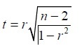    The null hypothesis is, of course, that the population correlation ρ=0
  • There are other measures of dependence such as Kendall’s ζ, Brownian correlation, Randomized Dependence Coefficient (RDC), entropy correlation, polychoric correlation, canonical correlation, and copula‐based dependence measures. These are less applicable in most empirical data and are not as popular or applicable in most situations.
  • The correlation matrix must be positive definite. That is, the correlation must be mathematically valid. For instance, suppose you are trying to correlate three variables: grades of graduate students in a particular year, the number of beers they consume a week, and the number of hours they study a week. One would assume that the following correlation relationships exist:
    • Grades and Beer (–) The more they drink, the lower the grades (no show on exams)
    • Grades and Study (+) The more they study, the higher the grades
    • Beer and Study (–) The more they drink, the less they study (drunk and partying all the time)

  However, if you input a negative correlation between Grades and Study, and assuming that the correlation coefficients have high magnitudes, the correlation matrix will be nonpositive definite. It would defy logic, correlation requirements, and matrix mathematics. However, smaller coefficients can sometimes still work even with the bad logic. When a nonpositive or bad correlation matrix is entered, Risk Simulator will automatically inform you and offer to adjust these correlations to something that is semi‐positive definite while still maintaining the overall structure of the correlation relationship (the same signs as well as the same relative strengths).

  • Finally, here are some notes in applying and analyzing correlations in Risk Simulator:
    • Risk Simulator uses the normal, T, and quasi‐normal copula methods to simulate correlated variable assumptions. The default is the normal copula, and it can be changed within the Risk Simulator | Options menu item. The T copula is similar to the normal copula but allows for extreme values in the tails (higher kurtosis events), and the quasi‐normal copula simulates correlated values between the normal and T copulas.
    • After setting up at least two or more assumptions, you can set correlations between pairwise variables by selecting an existing assumption and using the Risk Simulator | Set Input Assumption dialog.
    • Alternatively, the Risk Simulator | Analytical Tools | Edit Correlations menu item can be used to enter multiple correlations using a correlation matrix.
    • If historical data from multiple variables exist, by performing a distributional fitting using
      Risk Simulator | Analytical Tools | Distributional Fitting (Multi‐Variable), the report will automatically generate the best‐fitting distributions with their pairwise correlations computed and entered as simulation assumptions. In addition, this tool allows you to identify and isolate correlations that are deemed statistically insignificant using a twosample t‐test.
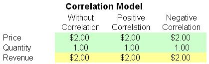
  FIGURE 1 Simple correlation model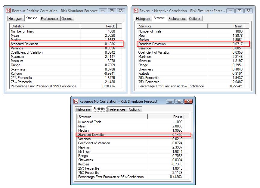
  FIGURE 2 Correlation results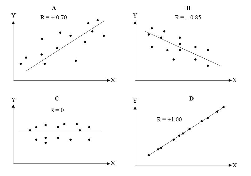
  FIGURE 3 Correlation of Simulated Values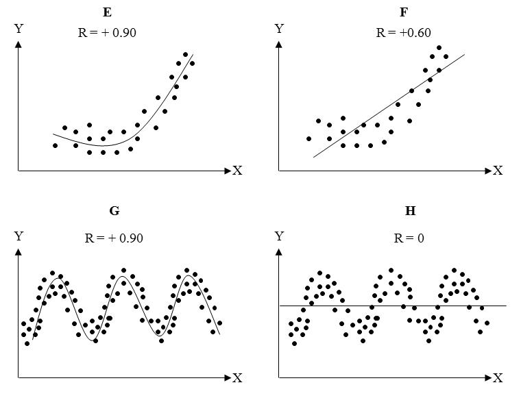
  FIGURE 4 Correlation of Simulated Values