The Pitfalls of Forecasting, Part 3

• By Admin
• September 3, 2014
• Comments Off on The Pitfalls of Forecasting, Part 3

Heteroskedasticity
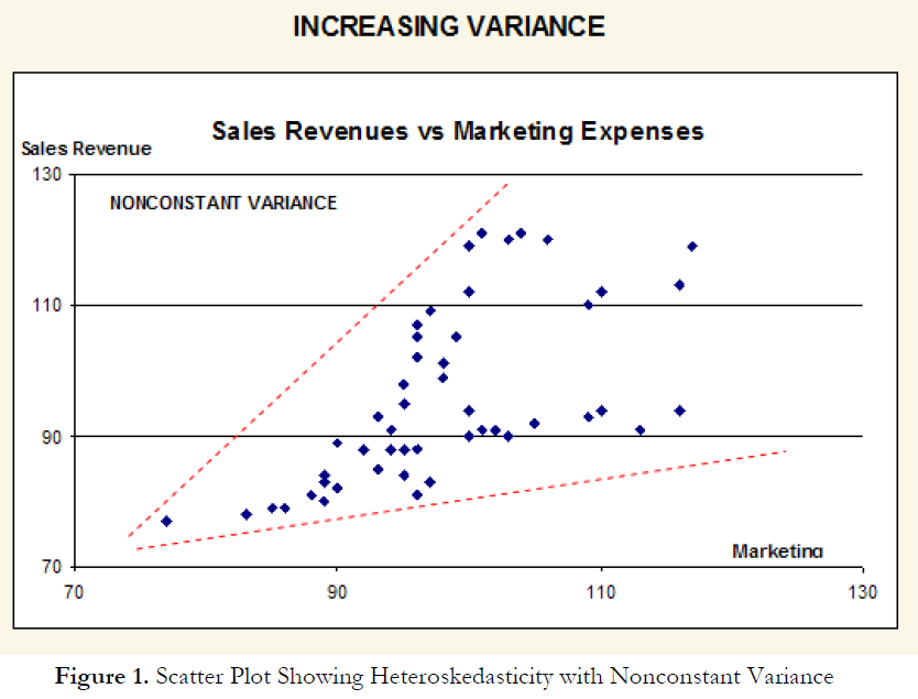
Another common problem encountered in time-series forecasting is heteroskedasticity; that is, the variance of the errors increases over time. Figure 1 illustrates this case, where the width of the vertical data fluctuations increases or fans out over time. In this example, the data points have been changed to exaggerate the effect. However, in most time-series analysis, checking for heteroskedasticity is a much more difficult task. If the variance of the dependent variable is not constant, then the error’s variance will not be constant.

The most common form of such heteroskedasticity in the dependent variable is that the variance of the dependent variable may increase as the mean of the dependent variable increases for data with positive independent and dependent variables. Unless the heteroskedasticity of the dependent variable is pronounced, its effect will not be severe: The least-squares estimates will still be unbiased, and the estimates of the slope and intercept will either be normally distributed if the errors are normally distributed, or at least normally distributed asymptotically (as the number of data points becomes large) if the errors are not normally distributed. The estimate for the variance of the slope and overall variance will be inaccurate, but the inaccuracy is not likely to be substantial if the independent-variable values are symmetric about their mean. Heteroskedasticity of the dependent variable is usually detected informally by examining the X-Y scatter plot of the data before performing the regression. If both nonlinearity and unequal variances are present, employing a transformation of the dependent variable may have the effect of simultaneously improving the linearity and promoting equality of the variances. Otherwise, a weighted least-squares linear regression may be the preferred method of dealing with nonconstant variance of the dependent variable.

Other Technical Issues
If the data to be analyzed by linear regression violate one or more of the linear regression assumptions, the results of the analysis may be incorrect or misleading. For example, if the assumption of independence is violated, then linear regression is not appropriate. If the assumption of normality is violated or outliers are present, then the linear regression goodness of fit test may not be the most powerful or informative test available, and this could mean the difference between detecting a linear fit or not. A nonparametric, robust, or resistant regression method; a transformation; a weighted least squares linear regression; or a nonlinear model may result in a better fit. If the population variance for the dependent variable is not constant, a weighted least-squares linear regression or a transformation of the dependent variable may provide a means of fitting a regression adjusted for the inequality of the variances. Often, the impact of an assumption violation on the linear regression result depends on the extent of the violation (such as how non-constant the variance of the dependent variable is, or how skewed the dependent variable population distribution is). Some small violations may have little practical effect on the analysis, while other violations may render the linear regression result useless and incorrect.

Other potential assumption violations include lack of independence in the dependent variable; independent variable random, not fixed; special problems with few data points (micronumerosity); and special problems with regression through the origin.

Lack of Independence in the Dependent Variable. Whether the independent-variable values are independent of eachother is generally determined by the structure of the experiment from which they arise. The dependent-variable values collected over time may be autocorrelated. For serially correlated dependent-variable values, the estimates of the slope and intercept will be unbiased, but the estimates of their variances will not be reliable and, hence, the validity of certain statistical goodness-of-fit tests will be flawed. An ARIMA model may be better in such circumstances.

The Independent Variable Is Random, Not Fixed. The usual linear regression model assumes that the observed independent variables are fixed, not random. If the independent values are not under the control of the experimenter (i.e., are observed but not set), and if there is, in fact, underlying variance in the independent variable, but they have the same variance, the linear model is called an errors-in-variables model or a structural model. The least-squares fit will still give the best linear predictor of the dependent variable, but the estimates of the slope and intercept will be biased (will not have expected values equal to the true slope and variance). A stochastic forecast model may be a better alternative here.

Special Problems with Few Data Points (Micronumerosity). If the number of data points is small (also termed micronumerosity), it may be difficult to detect assumption violations. With small samples, assumption violations such as nonnormality or heteroskedasticity of variances are difficult to detect even when they are present. With a small number of data points, linear regression offers less protection against violation of assumptions. With few data points, it may be hard to determine how well the fitted line matches the data, or whether a nonlinear function would be more appropriate.

Even if none of the test assumptions are violated, a linear regression on a small number of data points may not have sufficient power to detect a significant difference between the slope and zero, even if the slope is nonzero. The power depends on the residual error, the observed variation in the independent variable, the selected significance alpha level of the test, and the number of data points. Power decreases as the residual variance increases, decreases as the significance level is decreased (i.e., as the test is made more stringent), increases as the variation in observed independent variable increases, and increases as the number of data points increases. If a statistical significance test with a small number of data points produces a surprisingly non-significant probability value, then lack of power may be the reason. The best time to avoid such problems is in the design stage of an experiment, when appropriate minimum sample sizes can be determined, perhaps in consultation with an econometrician, before data collection begins.

Special Problems with Regression Through the Origin. The effects of non-constant variance of the dependent variable can be particularly severe for a linear regression when the line is forced through the origin: The estimate of variance for the fitted slope may be much smaller than the actual variance, making the test for the slope nonconservative (more likely to reject the null hypothesis that the slope is zero than what the stated significance level indicates). In general, unless there is a structural or theoretical reason to assume that the intercept is zero, it is preferable to fit both the slope and intercept.

Scatter Plots and Behavior of the Data Series
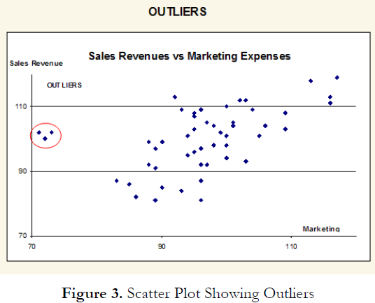
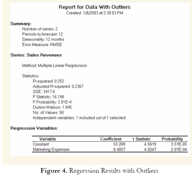
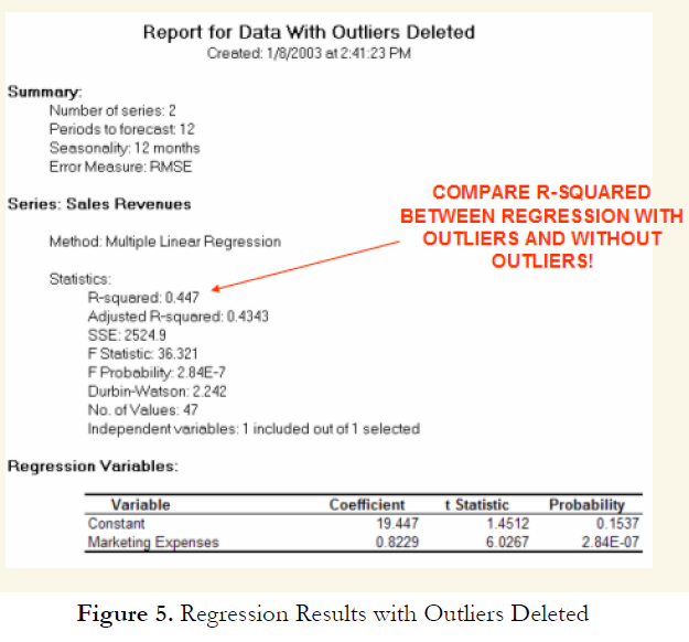
Other than being good modeling practice to create scatter plots prior to performing regression analysis, the scatter plot can also sometimes, on a fundamental basis, provide significant amounts of information regarding the behavior of the data series. Blatant violations of the regression assumptions can be spotted easily and effortlessly, without the need for more detailed and fancy econometric specification tests. For instance, Figure 3 shows the existence of outliers. Figure 4’s regression results, which include the outliers, indicate that the coefficient of determination is only 0.252 as compared to 0.447 in Figure 5 when the outliers are removed.

TO BE CONCLUDED IN “The Pitfalls of Forecasting, Part 4”