The Pitfalls of Forecasting, Part 4

• By Admin
• August 18, 2014
• Comments Off on The Pitfalls of Forecasting, Part 4

Scatter Plots and Behavior of the Data Series (continued)

As noted in “The Pitfalls of Forecasting, Part 3,” other than being good modeling practice to create scatter plots prior to performing regression analysis, the scatter plot can also sometimes, on a fundamental basis, provide significant amounts of information regarding the behavior of the data series. Blatant violations of the regression assumptions can be spotted easily and effortlessly, without the need for more detailed and fancy econometric specification tests.

When performing a regression analysis, values may not be identically distributed because of the presence of outliers. Outliers are anomalous values in the data and may have a strong influence over the fitted slope and intercept, giving a poor fit to the bulk of the data points. Outliers tend to increase the estimate of residual variance, lowering the chance of rejecting the null hypothesis. They may be due to recording errors, which may be correctable, or they may be due to the dependent-variable values not all being sampled from the same population. Apparent outliers may also be due to the dependent-variable values being from the same, but non-normal, population. Outliers may show up clearly in an X-Y scatter plot of the data, as points that do not lie near the general linear trend of the data. A point may be an unusual value in either an independent or dependent variable without necessarily being an outlier in the scatter plot.

The method of least squares involves minimizing the sum of the squared vertical distances between each data point and the fitted line. Because of this, the fitted line can be highly sensitive to outliers. In other words, least squares regression is not resistant to outliers, thus, neither is the fitted-slope estimate. A point vertically removed from the other points can cause the fitted line to pass close to it, instead of following the general linear trend of the rest of the data, especially if the point is relatively far horizontally from the center of the data (the point represented by the mean of the independent variable and the mean of the dependent variable). Such points are said to have high leverage: The center acts as a fulcrum, and the fitted line pivots toward high-leverage points, perhaps fitting the main body of the data poorly. A data point that is extreme in dependent variables but lies near the center of the data horizontally will not have much effect on the fitted slope, but by changing the estimate of the mean of the dependent variable, it may affect the fitted estimate of the intercept.

However, great care should be taken when deciding if the outliers should be removed. Although in most cases when outliers are removed, the regression results look better, a priori justification must first exist. For instance, if one is regressing the performance of a particular firm’s stock returns, outliers caused by downturns in the stock market should be included; these are not truly outliers as they are inevitabilities in the business cycle. Forgoing these outliers and using the regression equation to forecast one’s retirement fund based on the firm’s stocks will yield incorrect results at best. In contrast, suppose the outliers are caused by a single nonrecurring business condition (e.g., merger and acquisition) and such business structural changes are not forecast to recur; then these outliers should be removed and the data cleansed prior to running a regression analysis.

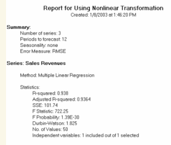
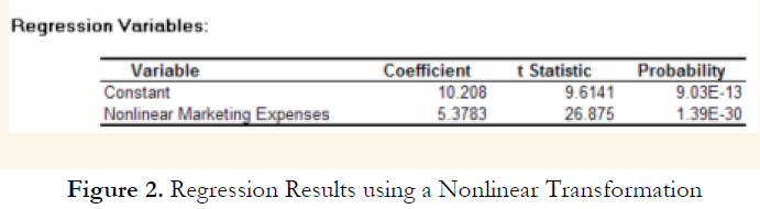
Figure 1 shows a scatter plot with a nonlinear relationship between the dependent and independent variables. In a situation such as this one, a linear regression will not be optimal. A nonlinear transformation should first be applied to the data before running a regression. One simple approach is to take the natural logarithm of the independent variable (other approaches include taking the square root or raising the independent variable to the second or third power) and regress the sales revenue on this transformed marketing-cost data series. Figure 2 shows the regression results with a coefficient of determination at 0.938, as compared to 0.707 in Figure 3 when a simple linear regression is applied to the original data series without the nonlinear transformation.

If the linear model is not the correct one for the data, then the slope and intercept estimates and the fitted values from the linear regression will be biased, and the fitted slope and intercept estimates will not be meaningful. Over a restricted range of independent or dependent variables, nonlinear models may be well approximated by linear models (this is, in fact, the basis of linear interpolation), but for accurate prediction, a model appropriate to the data should be selected. An examination of the X-Y scatter plot may reveal whether the linear model is appropriate. If there is a great deal of variation in the dependent variable, it may be difficult to decide what the appropriate model is; in this case, the linear model may do as well as any other, and has the virtue of simplicity.

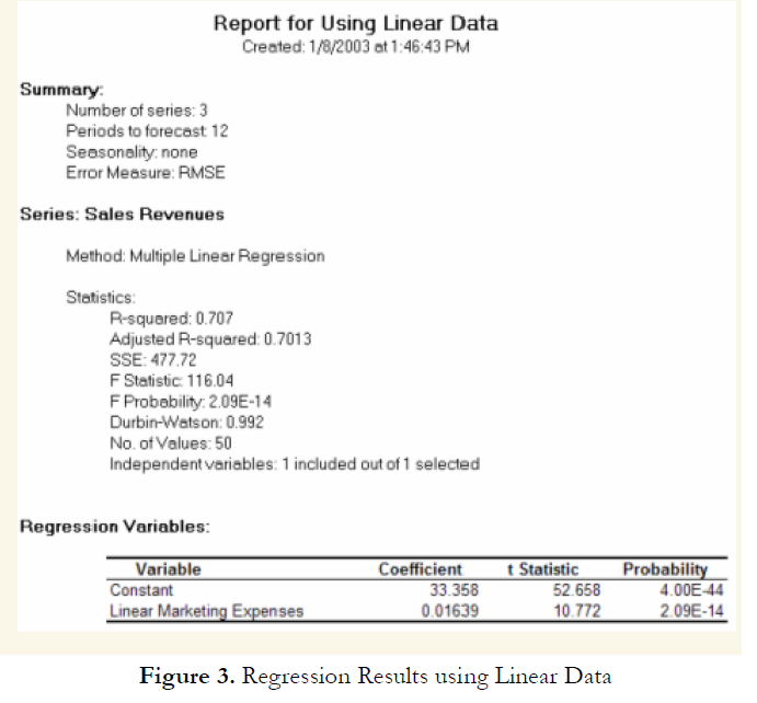
However, great care should be taken here as both the original linear data series of marketing costs should not be added with the nonlinearly transformed marketing costs in the regression analysis. Otherwise, multicollinearity occurs; that is, marketing costs are highly correlated to the natural logarithm of marketing costs, and if both are used as independent variables in a multivariate regression analysis, the assumption of no multicollinearity is violated and the regression analysis breaks down. Figure 4 illustrates what happens when multicollinearity strikes. Notice that the coefficient of determination (0.938) is the same as the nonlinear transformed regression (Figure 2). However, the adjusted coefficient of determination went down from 0.9364 (Figure 2) to 0.9358 (Figure 4). In addition, the previously statistically significant marketing-costs variable in Figure 2 now becomes insignificant (Figure 4) with a probability value increasing from close to zero to 0.4661. A basic symptom of multicollinearity is low t-statistics coupled with a high R-squared (Figure 4).