Time-Series Analysis

• By Admin
• December 15, 2014
• Comments Off on Time-Series Analysis

Theory
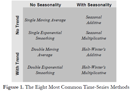
The eight most common time-series models, segregated by seasonality and trend, are shown in Figure
1. For instance, if the data variable has no trend or seasonality, then a single moving-average model or a single exponential-smoothing model would suffice. However, if seasonality exists but no discernible trend is present, either a seasonal additive or seasonal multiplicative model would be better, etc.

Procedure

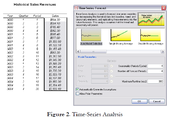
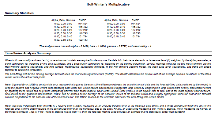
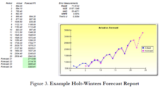
To follow along in this example, choose Auto Model Selection, enter 4 for seasonality periods per cycle, and forecast for 4 periods. Figure 3 shows the sample results generated by using the Forecasting tool. The model used was a Holt-Winters multiplicative model. Notice that in Figure 3, the model-fitting and forecast chart indicate that the trend and seasonality are picked up nicely by the Holt-Winters multiplicative model. The time-series analysis report provides the relevant optimized alpha, Beta, and gamma parameters; the error measurements; fitted data; forecast values; and forecast-fitted graph. The parameters are simply for reference. Alpha captures the memory effect of the base-level changes over time, Beta is the trend parameter that measures the strength of the trend, while gamma measures the seasonality strength of the historical data. The analysis decomposes the historical data into these three elements and then recomposes them to forecast the future. The fitted data illustrate the historical data and, using the recomposed model, show how close the forecasts are in the past (a technique called backcasting). The forecast values are either single-point estimates or assumptions (if the automatically generated assumptions option is chosen and if a simulation profile exists). The graph illustrates the historical, fitted, and forecast values. The chart is a powerful communication and visual tool to see how good the forecast model is.

This time-series analysis module contains the eight time-series models shown in Figure 1. You can choose the specific model to run based on the trend and seasonality criteria or choose the Auto Model Selection, which will automatically iterate through all eight methods, optimize the parameters, and find the best-fitting model for your data. Alternatively, if you choose one of the eight models, you can also deselect the Optimize checkboxes and enter your own alpha, Beta, and gamma parameters. In addition, you would need to enter the relevant seasonality periods if you choose the automatic model selection or any of the seasonal models. The seasonality input must be a positive integer (e.g., if the data is quarterly, enter 4 as the number of seasons or cycles a year, or enter 12 if monthly data, or any other positive integer representing the data periods of a full cycle). Next, enter the number of periods to forecast. This value also has to be a positive integer. The maximum runtime is set at 300 seconds. Typically, no changes are required. However, when forecasting with a significant amount of historical data, the analysis might take slightly longer and if the processing time exceeds this runtime, the process will be terminated. You can also elect to have the forecast automatically generate assumptions; that is, instead of single-point estimates, the forecasts will be assumptions. However, to automatically generate assumptions, a simulation profile must first exist. Finally, the polar parameters option allows you to optimize the alpha, Beta, and gamma parameters to include zero and one. Certain forecasting software allows these polar parameters while others do not. Risk Simulator allows you to choose which to use. Typically, there is no need to use polar parameters.