Understanding the Forecast Statistics and Four Moments

• By Admin
• July 7, 2014
• Comments Off on Understanding the Forecast Statistics and Four Moments

The Four Moments

Most distributions can be defined up to four moments. The first moment describes its location or central tendency (expected values); the second moment describes its width or spread (risks and uncertainties); the third moment, its directional skew (most probable events); and the fourth moment, its peakedness or thickness in the tails (catastrophic extreme tail events). All four moments should be calculated in practice and interpreted to provide a more comprehensive view of the project under analysis. Risk Simulator provides the results of all four moments in its Statistics view in the forecast charts.

Measuring the Center of the Distribution: The First Moment

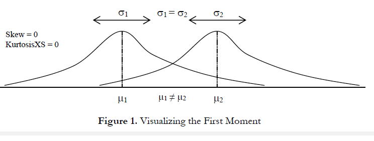
The first moment of a distribution measures the expected value or expected rate of return on a particular project. It measures the location of the project’s scenarios and possible outcomes on average. The common statistics for the first moment include the mean (average), median (center of a distribution), and mode (most commonly occurring value). Figure 1 illustrates the first moment––where, in this case, the first moment of this distribution is measured by the mean (µ), or average, value.

Measuring the Spread of the Distribution: The Second Moment

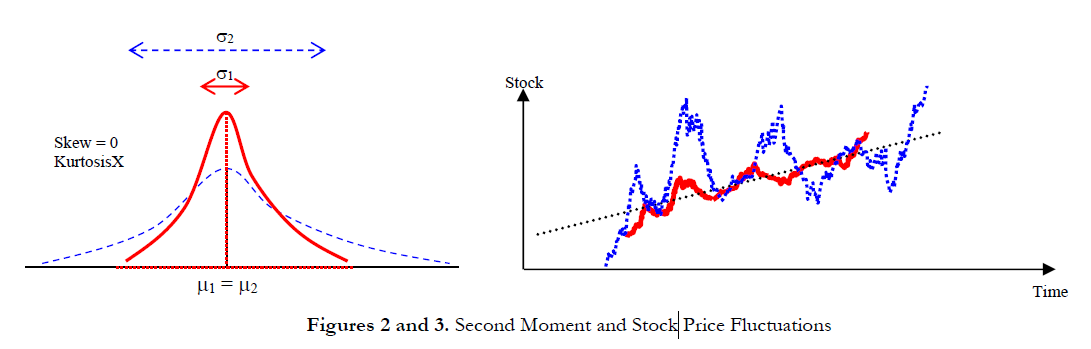
The second moment measures the spread of a distribution, which is a measure of risk. The spread, or width, of a distribution measures the variability of a variable, that is, the potential that the variable can fall into different regions of the distribution––in other words, the potential scenarios of outcomes. Figure 2 illustrates two distributions with identical first moments (identical means) but very different second moments or risks. The visualization becomes clearer in Figure 3, where as an example, suppose there are two stocks and the first stock’s movements (illustrated by the darker red line) with the smaller fluctuation is compared against the second stock’s movements (illustrated by the dotted blue line) with a much higher price fluctuation. Clearly an investor would view the stock with the wilder fluctuation as riskier because the outcomes of the more risky stock are relatively more unknown than the less risky stock. The vertical axis in Figure 3 measures the stock prices, thus, the more risky stock has a wider range of potential outcomes. This range is translated into a distribution’s width (the horizontal axis) in Figure 2, where the wider distribution represents the riskier asset. Hence, width, or spread, of a distribution measures a variable’s risks. Notice that in Figure 2, both distributions have identical first moments, or central tendencies, but clearly the distributions are very different. This difference in the distributional width is measurable. Mathematically and statistically, the width, or risk, of a variable can be measured through several different statistics, including the range, standard deviation (σ), variance, coefficient of variation, volatility, interquartile range, and percentiles.

Measuring the Skew of the Distribution: The Third Moment

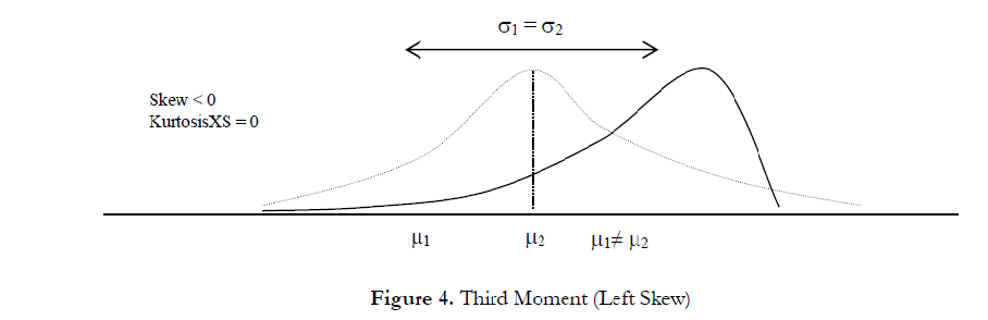
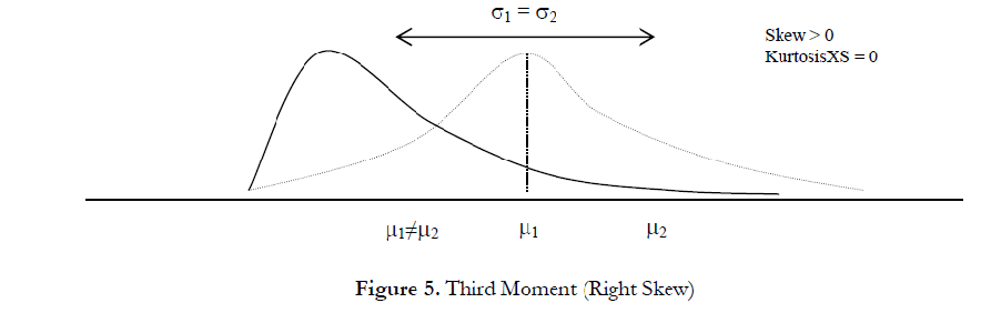
The third moment measures a distribution’s skewness, that is, how the distribution is pulled to one side or the other. Figure 4 illustrates a negative, or left, skew (the tail of the distribution points to the left) and Figure 5 illustrates a positive, or right, skew (the tail of the distribution points to the right). The mean is always skewed toward the tail of the distribution while the median remains constant. From another perspective, the mean moves but the standard deviation, variance, or width may still remain constant. If the third moment is not considered, then looking only at the expected value or expected returns (e.g., median or mean) and risk or uncertainty (standard deviation), a positively skewed project might be incorrectly chosen! For example, if the horizontal axis represents the net revenues of a project, then clearly a left or negatively skewed distribution might be preferred as there is a higher probability of greater returns (Figure 4) as compared to a higher probability for lower-level returns (Figure 5). Thus, in a skewed distribution, the median is a better measure of returns, as the medians for both Figures 4 and 5 are identical, risks are identical, and, hence, a project with a negatively skewed distribution of net profits is a better choice. Failure to account for a project’s distributional skewness may mean that the incorrect project may be chosen (e.g., two projects may have identical first and second moments, that is, they both have identical returns and risk profiles, but their distributional skews may be very different).

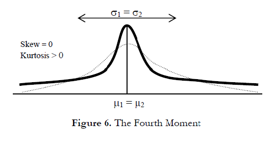
Measuring the Catastrophic Tail Events in a Distribution: The Fourth Moment

The fourth moment, or kurtosis, measures the peakedness of a distribution. Figure 6 illustrates this effect. The background (denoted by the dotted line) is a normal distribution with a kurtosis of 3.0, or an excess kurtosis (KurtosisXS) of 0.0. Risk Simulator’s results show the KurtosisXS value, using 0 as the normal level of kurtosis, which means that a negative KurtosisXS indicates flatter tails (platykurtic distributions like the Uniform or Triangular distributions), while positive values indicate fatter tails (leptokurtic distributions such as the Student’s T or Lognormal distributions). The distribution depicted by the bold line has a higher excess kurtosis, thus the area under the curve is thicker at the tails with less area in the central body. This condition has major impacts on risk analysis because for the two distributions in Figure 6, the first three moments (mean, standard deviation, and skewness) can be identical but the fourth moment (kurtosis) is different. This condition means that, although the returns and risks are identical, the probabilities of extreme and catastrophic events (potential large losses or large gains) occurring are higher for a high kurtosis distribution (e.g., stock market returns are leptokurtic, or have high kurtosis). Ignoring a project’s kurtosis may be detrimental. Typically, a higher excess kurtosis value indicates that the downside risks are higher (e.g., the Value at Risk of a project might be significant).

The Functions of Moments
Ever wonder why these risk statistics are called moments? In mathematical vernacular, moment means raised to the power of some value. In other words, the third moment implies that in an equation, three is most probably the highest power. In fact, the following equations illustrate the mathematical functions and applications of some moments for a sample statistic. For example, notice that the highest power for the first moment average is one, the second moment standard deviation is two, the third moment skew is three, and the highest power for the fourth moment is four.

First Moment: Arithmetic Average or Simple Mean (Sample). The Excel equivalent function is AVERAGE.

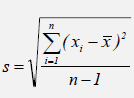
Second Moment: Standard Deviation (Sample). The Excel equivalent function is STDEV for a sample standard deviation.
The Excel equivalent function is STDEVP for a population standard deviation.

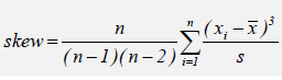
Third Moment: Skew. The Excel equivalent function is SKEW.

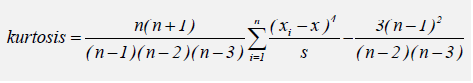
Fourth Moment: Kurtosis. The Excel equivalent function is KURT.

The Measurements of Risk
There are multiple ways to measure risk in projects. This section summarizes some of the more common measures of risk and lists their potential benefits and pitfalls.

Probability of Occurrence
This approach is simplistic yet effective. As an example, there is a 10% probability that a project will not break even (it will return a negative net present value indicating losses) within the next 5 years. Further, suppose two similar projects have identical implementation costs and expected returns. Based on a single-point estimate, management should be indifferent between them. However, if risk analysis such as Monte Carlo simulation is performed, the first project might reveal a 70% probability of losses compared to only a 5% probability of losses on the second project. Clearly, the second project is better when risks are analyzed. Standard Deviation and Variance Standard deviation is a measure of the average of each data point’s deviation from the mean. This is the most popular measure of risk, where a higher standard deviation implies a wider distributional width and, thus, carries a higher risk. The drawback of this measure is that both the upside and downside variations are included in the computation of the standard deviation. Some analysts define risks as the potential losses or downside; thus, standard deviation and variance will penalize upswings as well as downsides. Semi-Standard Deviation The semi-standard deviation only measures the standard deviation of the downside risks and ignores the upside fluctuations. Modifications of the semi-standard deviation include calculating only the values below the mean or values below a threshold (e.g., negative profits or negative cash flows). This provides a better picture of downside risk but is more difficult to estimate.

Volatility
The concept of volatility is widely used in the applications of real options and can be defined briefly as a measure of uncertainty and risks. Volatility can be estimated using multiple methods, including simulation of the uncertain variables impacting a particular project and estimating the standard deviation of the resulting asset’s logarithmic returns over time. This concept is more difficult to define and estimate but more powerful than most other risk measures in that this single value incorporates all sources of uncertainty rolled into one value.

Beta
Beta is another common measure of risk in the investment finance arena. Beta can be defined simply as the undiversifiable, systematic risk of a financial asset. This concept is made famous through the CAPM, where a higher Beta means a higher risk, which in turn requires a higher expected return on the asset.

Coefficient of Variation
The coefficient of variation is simply defined as the ratio of standard deviation to the mean, where risks are commonsized. For example, a distribution of a group of students’ heights (measured in meters) can be compared to the distribution of the students’ weights (measured in kilograms). This measure of risk or dispersion is applicable when the variables’ estimates, measures, magnitudes, or units differ.

Value at Risk (VaR)
Value at Risk was made famous by J. P. Morgan in the mid-1990s through the introduction of its RiskMetrics approach, and has thus far been sanctioned by several bank governing bodies around the world. Briefly, it measures the amount of capital reserves at risk given a particular holding period at a particular probability of loss. This measurement can be modified to risk applications by stating, for example, the amount of potential losses a certain percentage of the time during the period of the economic life of the project––clearly, a project with a smaller VaR is better.

Worst-Case Scenario and Regret
Another simple measure is the value of the worst-case scenario given catastrophic losses, or regret. That is, if a decision is made to pursue a particular project, but if the project becomes unprofitable and suffers a loss, the level of regret is simply the difference between the actual losses compared to doing nothing at all.

Risk-Adjusted Return on Capital
Risk-adjusted return on capital (RAROC) takes the ratio of the difference between the fiftieth percentile (median) return and the fifth percentile return on a project to its standard deviation. This approach is used mostly by banks to estimate returns subject to their risks by measuring only the potential downside effects and ignoring the positive upswings.